Francisco Romaldo Fernandes MendesHexohttps://franciscormendes.com/gallery/favicon-32x32.pnghttps://franciscormendes.com/All rights reserved 2026, Francisco Romaldo Fernandes MendesFrancisco Mendes2026-05-21T15:47:38.225ZFrancisco Romaldo Fernandes MendesBackground
This blog post was spurred by an interesting discussion with a coworker of mine. The question was relatively simple, “why do we use graphs for recommender systems, why not just use tabular ML?”. This question caused a sort of existential crisis in me, somewhat more than the average Murakami character (in the first 10 chapters). We will use a strategy that is commonly used across mathematics, we will show that something is a simplified version of something else. In order to do this we need to have a principled way of thinking about recommender systems.
Basic Math of Recommender Systems
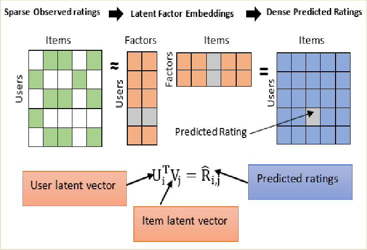
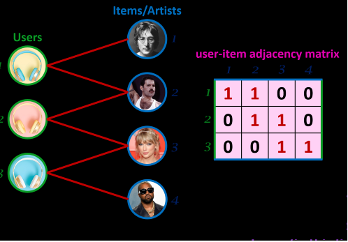
The most general way to think about a recommender system is to actually think of it in terms of products x users. This is either the adjacency matrix for the graph or the matrix to be factorized for the matrix factorization approach. So let us create this,
Here $U$ is a $5 \times 2$ matrix of movie embeddings and $V^\top$ is a $2 \times 4$ matrix of user embeddings, where 2 is the number of latent factors. The entries of $\hat{A}$ will not necessarily be 1s and 0s but rather as close as possible, minimising:
where $u_i$ and $v_j$ are the rows of $U$ and $V$ corresponding to movie $m_i$ and user $u_j$. Defining $e_{ij} = A_{ij} - u_i \cdot v_j$, gradient descent updates each embedding by nudging it in the direction that reduces the error:
In the GCN approach we treat movies and users as nodes in a bipartite graph. An edge connects movie $m_i$ to user $u_j$ whenever $A_{ij} = 1$. We stack these into a single $(5+4) \times (5+4)$ adjacency matrix:
The top-right block is the movie-to-user interactions from $A$; the bottom-left is its transpose. There are no movie-movie or user-user edges.
Before propagating information we symmetrically normalise $R$ by the degree matrix $D$, where $D_{ii} = \sum_j R_{ij}$:
$$\hat{R} = D^{-1/2} \, R \, D^{-1/2}$$
A single GCN aggregation layer then updates every node’s embedding by averaging its neighbours’ and applying a learnable weight matrix $W^{(0)}$:
$$E^{(1)} = \hat{R} \, E^{(0)} \, W^{(0)}$$
where $E^{(0)} \in \mathbb{R}^{9 \times d}$ is a matrix of initial node embeddings (one row per node, $d$ dimensions). After one pass, a movie node’s new embedding is a weighted average of the embeddings of the users who watched it, and vice versa. This is the key structural difference from matrix factorisation: instead of fitting two flat factor matrices independently, the GCN lets each node gather information from its neighbours before a prediction is made.
In the matrix factorisation case we get $U$ and $V$, separate movie and user embedding matrices. The GCN produces the same thing, but because of the structure of $R$ both sets of embeddings live in a single matrix $E^{(0)}$: movie rows stacked on top of user rows. The rank of this matrix, like the number of latent factors in matrix factorisation, is the number of columns $d$. Both $E^{(0)}$ and $W^{(0)}$ are learned via backpropagation by minimising the error between the predicted and observed interactions:
where $e_{u_j}$ and $e_{m_i}$ are the rows of $E^{(1)}$ corresponding to user $u_j$ and movie $m_i$.
Recap
In both cases you get a matrix of vectors of shape $(m+n) \times d$, where each row is a latent representation of either a movie or a user. The idea is that if we can represent movies and users in a shared latent space such that similar movies and users are closer together, then predicting an interaction between a user and a movie they have not seen before is trivial, simply take the dot product of their latent representations and you have a number that tells you how likely they are to interact. Notice that you are learning these representations solely by looking at who watched which movies.
What if I have a representation that I want to use?
After learning that all the recommender system tries to do is find a latent representation of a user and a movie, you might say, hang on a minute, I actually know of an overt (as in NOT latent) representation that already places similar users close together. For example, suppose a user filled out a form asking what genres of movies they are interested in, and answered honestly. Would that not also place users with the same preferences closer together? With the added advantage that this is something they have explicitly told you?
That is a fair point. It turns out you can incorporate those explicit features alongside the latent ones, you learn weights for both the latent embeddings and the explicit features, and you also learn the embeddings themselves. The only thing you do not update are the feature columns in $X$, since those are representations you already trust. Think of it as freezing the columns you know are good and letting the model learn everything else around them.
Matrix case
Suppose each movie $m_i$ has a feature vector $x_{m_i} \in \mathbb{R}^p$ (e.g. genre indicators) and each user $u_j$ has a feature vector $x_{u_j} \in \mathbb{R}^q$ (e.g. stated genre preferences). We can augment the latent factor prediction with explicit features:
where $\beta_m \in \mathbb{R}^p$ and $\beta_u \in \mathbb{R}^q$ are learned coefficient vectors. The loss sums over all observed pairs (both 1s and 0s), where $\Omega$ denotes the set of observed entries in $A$:
where $e_{ij} = y_{ij} - \hat{y}_{ij}$. The structure is identical to the latent factor case. The only difference is that $x_{m_i}$ and $x_{u_j}$ are fixed observed features rather than vectors being learned from scratch.
GCN case
The GCN equivalent keeps the latent and feature streams separate, each with its own weight matrix:
The graph propagation enriches both streams: after one aggregation step, each node’s embedding is a weighted average of its neighbours’ latent and feature representations independently transformed before being summed.
Conclusion
The two prediction equations summarise everything, and the pure latent models fall out as special cases:
Using only the interaction matrix is not a different class of model. It is the full model with the feature coefficients constrained to zero ($\beta_m, \beta_u = 0$ in the MF case and $W_{\text{features}} = 0$ in the GCN case).
Appendix
What is $E^{(0)}$?
$E^{(0)}$ is a randomly initialised matrix where each entry is sampled from a standard normal distribution.
How does the loss function use $R$?
$R$ plays two distinct roles during training.
1. Graph structure for propagation. $\hat{R}$ defines which nodes aggregate from which neighbours at every forward pass, exactly as shown above.
2. Source of training signal. The entries of $R$ are the labels. For a given user $u_j$ and movie $m_i$, the predicted score is the dot product of their final embeddings:
$$\hat{y}_{ij} = e_{u_j} \cdot e_{m_i}$$
and the ground truth is simply $y_{ij} = R_{ij} = 1$ for every observed interaction. The loss penalises the difference between the two across all observed pairs:
Minimising this loss via backpropagation shapes $E^{(0)}$ so that users end up close in embedding space to the items they have interacted with. $R$ is therefore both the adjacency matrix that drives message passing and the labelled dataset that supervises learning.
When to Use a Graph Versus Tabular ML for Recommender Systems?2026-05-21T15:47:38.225ZFrancisco Romaldo Fernandes MendesDisclaimer: the scenario described in this article is entirely fictional. Any resemblance to actual experiments, programs, or conversations is coincidental. The math, however, is real.
The Setup
Imagine you are running an experiment to test the efficacy of a rewards program built to incentivize the use of autonomous vehicles in a ride-share marketplace. AVs cost more to operate than driver cars (for now; this is largely due to logistical issues that will likely be solved by scale), so the business case depends heavily on whether riders can be nudged toward them at sufficient volume. The rewards program is the nudge and you need to know if it works.
The rewards program costs money for every day it runs. Every subsidised ride is a line item. So there is real pressure to end the experiment as early as possible. Enter a Bayesian disciple who proposes a solution: run a Bayesian experiment instead of a frequentist one. The argument is that Bayesian methods allow you to check results continuously and stop the moment you have sufficient evidence, dispensing with the need for a fixed sample size, the indignity of waiting, and crucially the problem of peeking, that is, the practice of inspecting results before the planned sample size is reached and stopping early if the numbers look good, which inflates your false positive rate.
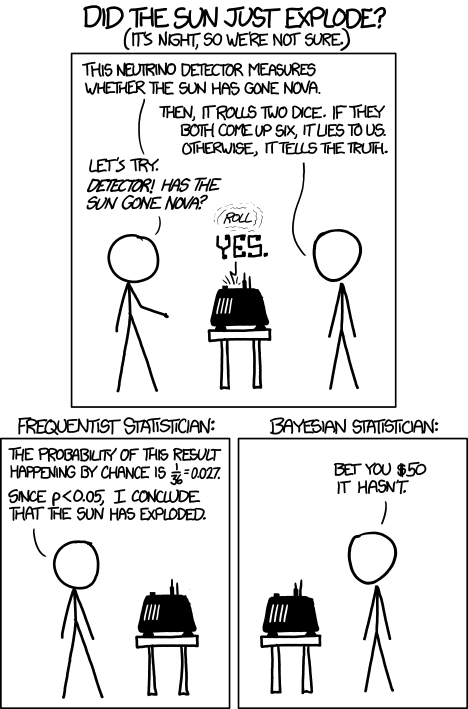
XKCD #1132: Frequentists vs. Bayesians (Randall Munroe, CC BY-NC 2.5). The Bayesian in this comic is right about priors. The Bayesian in our meeting was right about priors too. Neither of them was right about the experiment being cheap.
The proposal was reasonable and well-intentioned. My concern was specific, and asserting it without proof felt insufficient, so I brought the math.
Frequentist Sample Size
To set the baseline, here is the standard frequentist formulation. We are testing whether the rewards program (treatment) increases AV ride take-rate relative to no rewards (control), where $\theta$ is the probability a rider chooses an AV and $\Delta = \theta_T - \theta_C$ is the MDE:
$$H_0: \Delta = 0, \quad H_1: \Delta > 0$$
With Type I error $\alpha$ and power $1-\beta$, the required sample size per group is:
where $z_q$ denotes the $q$-th quantile of the standard normal distribution. The numerator grows with the variance of each group; the denominator shrinks with the MDE squared. If the rewards program moves the AV take-rate only slightly, $\Delta$ is small, the required sample size is large, and the program runs at a loss for a long time. This was the source of the pressure: the expected MDE was small, the required sample size was large, and every additional day of the experiment was another line item.
This is the formula the Bayesian disciple proposed to improve upon. On to the proposed alternative.
Bayesian Sample Size
The Bayesian formulation replaces the frequentist error guarantees with a posterior expected loss criterion. We approximate the posterior on each group’s conversion rate as Gaussian, which is reasonable for proportions with sufficient data:
where $\hat{\Delta} = \hat{\theta}_T - \hat{\theta}_C$ is the estimated MDE and $\Phi^{-1}$ is the inverse standard normal CDF. Look at the structure. It is identical to the frequentist formula. The variance terms are the same. The MDE in the denominator is the same. The only difference is the squared prefactor: $\left[\Phi^{-1}(1-\epsilon)\right]^2$ instead of $\left(z_{1-\alpha/2} + z_{1-\beta}\right)^2$.
Example
Put some numbers on it. Suppose the baseline AV take-rate is 50% and the rewards program is expected to lift it by 2 percentage points:
On paper, the Bayesian approach needs roughly a third of the frequentist sample. It is an appealing result, and the intuition behind it is sound. There is just one assumption buried in the derivation that changes everything.
Bayesian Is Not Immune to Peeking
For the uninitiated, peeking is the practice of inspecting results before the planned sample size is reached and stopping early if the numbers look good. It is what invalidates frequentist tests when p-values are checked repeatedly mid-experiment: the false positive rate inflates because you are effectively running multiple tests and keeping the best result. The same logic applies to the Bayesian posterior.
You might be tempted to think you can check the Bayesian experiment after every ride or every day. This is incorrect: you still need to let $n_\text{bayes}$ observations accumulate before evaluating the stopping criterion, otherwise this is also peeking. Bayesian methods have an additional problem here: the posterior variance can jump around quite a bit early on, so making a decision off it is unreliable. In other contexts such as the Kalman filter, this period of instability would be called burn-in.
If you evaluate $p_\text{wrong} < \epsilon$ continuously and stop the moment it dips below threshold, you have not run the experiment described by the formula above. You have run something different, with different and worse statistical properties. The Bayesian framing does not make this problem disappear. It reframes it. The stopping rule is still a rule, and it must be respected as such.
When Are the Two Formulas Exactly the Same?
The two formulas have identical structure: same variance terms, same MDE in the denominator. The only difference is the prefactor. Setting them equal gives:
Plug in the numbers from the example above: $\alpha = 0.05$, power $= 0.8$, so $z_{1-\alpha/2} + z_{1-\beta} = 2.8$. Then:
$$\epsilon^* = 1 - \Phi(2.8) \approx 0.0026$$
This is what it means. For the Bayesian experiment to require the same sample size as the frequentist one, you must set $\epsilon = 0.26\%$, not the $5\%$ used in the earlier example. The apparent sample size reduction comes entirely from setting a far more lenient $\epsilon$. When you hold the error guarantees constant across both frameworks, the sample sizes are exactly equal.
It is worth noting that the relationship between $\epsilon$ and the frequentist parameters $\alpha$ and $\beta$ is not always this transparent. Under the Gaussian approximation used here, the algebra works out cleanly. For other likelihood models or more complex posteriors, deriving the equivalent $\epsilon^*$ requires its own careful analysis and the equivalence will not always take such a neat closed form. The general principle, however, tends to hold: when you account for what each framework is actually guaranteeing, no free lunch is to be found.
Conclusion
The Bayesian framework is not buying a smaller experiment. It is buying a different interpretation of the same data, at the same cost, with the same number of subsidised AV rides. If the goal is to reduce experiment duration, the honest levers are: a larger MDE (better rewards design), higher tolerance for error, or lower power. Choosing a different statistical framework is not one of them.
Appendix: Burn-In in the Kalman Filter
A Kalman filter is an algorithm for tracking a hidden quantity (say, the position of a vehicle) by combining noisy sensor readings with a prior belief about where the vehicle was a moment ago. At each time step it updates its estimate and, crucially, its uncertainty about that estimate.
The problem is that the filter needs to be initialised somewhere. If you start it with a poor guess, or simply with a very diffuse prior because you genuinely do not know, the first several estimates will be unreliable. The posterior variance is large, the estimate is sensitive to whatever noisy observation came in first, and the filter has not yet had enough data to correct itself. This settling period is called burn-in. Practitioners routinely discard these early estimates and only trust the filter’s output once the variance has stabilised.
The parallel to a Bayesian experiment is direct. In the early observations, the posterior over your treatment effect is similarly volatile, dominated by the prior and highly sensitive to the first few data points. A posterior that crosses your threshold on day two is not evidence the treatment works; it is the filter still finding its feet. Waiting for $n_\text{bayes}$ is the experiment’s equivalent of discarding the burn-in period.
Johari, R., Pekelis, L., & Walsh, D. (2015). Always Valid Inference: Bringing Sequential Analysis to A/B Testing. arXiv:1512.04922.
]]>
https://franciscormendes.com/2026/04/10/bayesian-vs-frequentist-sample-size/2026-04-10T04:00:00.000ZAn AV rewards program, a Bayesian disciple, and the claim that Bayesian experiments let you peek. They do not. Here is the math.Bayesian Peeking is Still Peeking: Rigorous Proof, No Priors Required2026-05-20T16:32:39.866ZFrancisco Romaldo Fernandes MendesIntroduction
In autonomous driving, perception systems typically rely on photons i.e. cameras, lidar, and radar. But what if we could also listen to the environment, capturing sound cues that are invisible to traditional vision-based sensors?
There are many intuitively appealing use cases where an additional sensing modality could enhance awareness of the surroundings. Acoustic sensing itself is not new in automotive systems. For example, ultrasonic sensors have long been used for short-range applications such as parking assistance. Extending this idea to environmental sound sensing—allowing a vehicle to effectively hear its surroundings—has been explored by organizations such as the Fraunhofer Institute and Renesas Electronics. At CVPR ‘23 we had the Princeton Computational Image lab create 2D “images” using beamforming (more on this later) from passive acoustic listening and fused this with RGB camera data.
While the Princeton paper was highly influential to this work, our client was interested in passing certain scenarios only without overly relying on (or expending energy on) a highly complex multi-dimensional sensor modality. In this post we explore several motivations for adding a simpler version of passive acoustic sensing to the autonomous vehicle sensor stack.
Sneak Peek of our solution: Flashing red/cyan vehicle is emitting sound
Why consider acoustic sensing?
Obstructed-view scenarios are increasingly emphasized in safety standards such as Euro NACP. Detecting hazards before they become visible is critical for improving safety metrics.
With the rise of autonomous systems in defense and security applications, additional sensing modalities may provide a differentiator when competing for contracts.
Sound does not require line-of-sight (LoS). Important events such as children playing in the street, emergency vehicle sirens, or approaching traffic can be detected even when visually occluded.
Sound is a natural communication modality for humans, and could provide a mechanism for richer interaction between the environment and the ego vehicle.
Acoustic signals can intrinsically provide directional information (heading), which can improve situational awareness metrics such as MAPH (Mean Average Precision with Heading).
Beamforming+RGB outperforms RGB alone in challenging occluded scenarios
Key disadvantages
Acoustic sensing also introduces several challenges:
Passive acoustic systems typically provide Angle-of-Arrival (AoA) information but not reliable distance estimates.
Performance can degrade due to vehicle noise, wind noise, and environmental interference.
Toy Example: Acoustic Direction Improves Early Detection
To illustrate the value of acoustic sensing, consider a simple scenario:
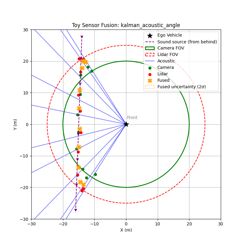
An emergency vehicle approaches from the bottom-right relative to the ego vehicle.
Acoustic sensing estimates the direction of arrival using TDOA between microphones, but cannot determine distance.
Camera and lidar only detect the vehicle once it enters their field of view.
In the simulation, the vehicle moves toward the ego vehicle. The acoustic system continuously estimates a sextant, or directional sector, while the camera and lidar begin detecting the vehicle only after it enters their sensing range.
This allows the fusion system to gain early directional awareness, giving planning systems a chance to anticipate the approaching vehicle before visual confirmation. Even though the acoustic angle estimate is noisy, it provides information beyond the field of view of both camera and lidar. After fusing with lidar and camera data, the system produces more accurate position estimates.
Context
The work described here was originally developed at Reality AI, which was later acquired by Renesas Electronics to explore the commercial feasibility of passive acoustic sensing in automotive systems. My role focused on scaling the solution and validating it across different environments.
We conducted experiments using simulated emergency sirens in multiple environments, including:
controlled warehouse setups
busy urban streets
open environments with realistic traffic noise
We also collaborated with external partners to collect additional datasets and explore multi-sensor fusion approaches.
In this article, I will explore PAMVON (Passive Acoustic Monitoring for Vehicles and Objects)—a system that uses microphone arrays, signal processing, and machine learning to detect and localize important acoustic events in the driving environment.
The work described here was originally developed at Reality AI, which was later acquired by Renesas Electronics to explore the commercial feasibility of passive acoustic sensing in automotive systems. My role focused on scaling the solution and validating it across different environments.
We conducted experiments using simulated emergency sirens in multiple environments, including:
controlled warehouse setups
busy urban streets
open environments with realistic traffic noise
We also collaborated with external partners to collect additional datasets and explore multi-sensor fusion approaches.
Passive Acoustic Monitoring (PAM)
Passive Acoustic Monitoring (PAM) detects environmental sounds without emitting signals. Instead, the system passively listens for events in the surrounding environment such as emergency vehicle sirens, horns, tire skids, engine noise, drones or machinery, and even children playing in the street.
The key advantage of this approach is that sound does not require line-of-sight. Important cues can be detected even when they are visually occluded, in low-light conditions, or in adverse weather. This makes acoustic sensing particularly attractive for early warning scenarios, such as an approaching ambulance that has not yet entered the field of view of the vehicle’s cameras or lidar.
Recent developments in multimodal large language models also change how one might think about acoustic perception. Rather than requiring a rigid classifier that assigns each sound to a predefined category, modern multimodal systems can reason over audio signals more flexibly and incorporate them into a broader contextual understanding of the scene. In practice this means the acoustic signal can act less as a strict classification task and more as an additional stream of environmental information that the perception system can interpret alongside vision and other sensor modalities.
Microphone Arrays and Beamforming
Sound (like light) travels in a straight line and therefore we need at least 4 microphones to provide an accurate estimate of the angle of arrival of the sound wave. A single microphone provides limited spatial information. To estimate where a sound originates, passive acoustic monitoring systems typically use small arrays of microphones. By observing the time differences between when a signal reaches each microphone, the system can estimate the direction of arrival of the sound source. Arrays also make it possible to improve signal quality by combining signals from multiple sensors.
In practice this enables several useful capabilities. The system can estimate the direction of arrival of a sound, approximate the location of the source under certain assumptions, and improve the signal-to-noise ratio by combining measurements across the array.
Beamforming is the signal processing technique that makes this possible. The idea is simple: signals arriving from a particular direction reach each microphone at slightly different times. By applying the appropriate delays and summing the signals together, the array reinforces sounds from the desired direction while suppressing sounds from other directions.
In practice the system estimates the relative delay between microphones using cross-correlation. When a sound arrives at the array, it reaches each microphone at slightly different times. By computing the cross-correlation between pairs of microphone signals, the system can estimate the time difference of arrival between them.
These time differences constrain the direction from which the sound could have originated. With multiple microphone pairs, the system can estimate a consistent direction of arrival for the source.
Once the delays are known, the array can also combine the microphone signals in a way that reinforces sounds coming from that direction while suppressing others. In effect, the array behaves like a steerable listening sensor that can focus on different parts of the acoustic scene.
Angle of Arrival (AoA) Estimation via Cross-Correlation
In a microphone array, a sound source reaches each microphone at slightly different times. By comparing these signals, the system can estimate the relative delay between them. A common way to do this is through cross-correlation, which measures how similar two signals are as one is shifted in time relative to the other.
For two microphone signals $x_1(t)$ and $x_2(t)$, the cross-correlation can be written as
In real environments, reflections and background noise can make the correlation peak less reliable. A commonly used approach to improve robustness is generalized cross-correlation with phase transform (GCC-PHAT). This method emphasizes phase information in the frequency domain and reduces the influence of signal magnitude differences:
Here $X_1(f)$ and $X_2(f)$ are the Fourier transforms of the microphone signals. The peak of $R_{12}(\tau)$ provides a stable estimate of the arrival delay, which can then be used to infer the direction of the sound source.
Signal Processing Pipeline
Passive acoustic monitoring typically follows a structured processing pipeline:
Preprocessing: The raw microphone signals are filtered to remove irrelevant frequency bands, and gain normalization ensures consistent amplitude levels across microphones.
Time-frequency analysis: Signals are converted into spectrograms using the Short-Time Fourier Transform (STFT), revealing how frequency content evolves over time.
Beamforming: Directional enhancement techniques, such as delay-and-sum or cross-correlation-based beamforming, focus on sounds from specific directions while suppressing noise and interference.
Event detection: Open-source neural networks, including VGGish, convolutional-recurrent networks (CRNNs), and transformers, analyze the spectrograms to detect and classify events such as sirens, horns, or tire skids.
Localization: Time Difference of Arrival (TDOA) estimates, often computed using GCC-PHAT cross-correlation, are combined across microphone pairs to infer the direction of incoming sounds and, in some cases, approximate source locations.
This pipeline allows the system to transform raw audio into actionable information for autonomous vehicle perception, providing early warning of hazards even when they are outside the line of sight of cameras or lidar.
Acoustic Sensor Data Representation
In a generalized form, data from a passive acoustic monitoring array can be represented as a tuple capturing the relevant information for fusion:
$\theta$: Estimated angle of arrival (AoA) of the sound, typically computed using TDOA and cross-correlation (GCC-PHAT).
$\sigma_\theta$: Uncertainty of the angle estimate, reflecting noise, reverberation, or low SNR.
$c$: Sound class probability vector produced by the ML model. The classes correspond to ambulance, police, and other unknown loud sounds. For example, $c = [0.7, 0.2, 0.1]$
$f$: Frequency-domain features, such as Mel spectrogram or STFT frame, optionally used for downstream ML fusion.
$t$: Timestamp of the measurement, to allow temporal alignment with other sensors.
$\mathbf{p}_{\text{ego}}$: Pose of the ego vehicle when the measurement was captured, typically $(x, y, \psi)$ in 2D or 3D coordinates.
This representation allows the acoustic signal to integrate easily into perception and fusion pipelines:
$\theta$ provides a directional prior for early detection.
$c$ informs semantic understanding of the source.
$\sigma_\theta$ can be used in probabilistic fusion (e.g., weighted averaging, Kalman updates).
$f$ allows future retraining or fine-tuning of ML models.
$t$ and $\mathbf{p}_{\text{ego}}$ allow projection into bird’s-eye view (BEV) maps or occupancy grids alongside camera and lidar data.
For an array of $N$ microphones, the raw signals can also be stored as:
These raw signals are processed into the generalized form above, providing a compact yet rich representation for sensor fusion.
Simple ID-Based Matching
Before exploring a more technical late fusion approach, we first evaluated a simpler strategy based on ID matching. In this setup, acoustic detections were associated directly with annotated object identities in the dataset.
The acoustic classifier produced class probabilities for events such as ambulance sirens, police sirens, or other loud sounds. When the classifier detected a high probability ambulance siren, we matched that event to the corresponding object detection annotation in the scene. In practice this meant associating the acoustic event with the object ID labeled as an emergency vehicle in the perception dataset.
One challenge is that the acoustic detector often produces a directional estimate much earlier than the moment when the vehicle becomes visible and is annotated by the vision system. The acoustic pipeline provides an angle of arrival $\theta$, but not a direct range estimate. To place this information in the BEV representation, we projected the acoustic bearing into the map by creating an artificial point along the direction of arrival at a fixed distance $d$ from the ego vehicle. The distance was chosen to be larger than the field of view of the camera and lidar sensors so that the acoustic signal could represent a potential source outside the current perception range.
where $(x_{ego}, y_{ego})$ is the position of the ego vehicle in BEV coordinates. As the vehicle approaches and eventually enters the sensor field of view, the projected acoustic point becomes spatially consistent with the detected object.
This approach relies on the object detection pipeline already identifying vehicles and assigning consistent IDs across frames. The acoustic system then acts as an additional signal that confirms the presence of a specific type of vehicle.
Although simple, this method is surprisingly effective. The acoustic cue provides early detection of emergency vehicles, while the vision system provides precise localization and tracking. By linking the acoustic classification to existing object IDs, the system can quickly identify which tracked object is likely producing the sound.
This ID-based matching served as a useful baseline before implementing a more general late fusion approach using probabilistic tracking and bearing measurements.
Late Fusion with an Existing BEV Pipeline
While the ID-based matching approach provided a strong baseline, it relies on the object already being detected and assigned an identity by the perception pipeline. In many cases the acoustic signal appears earlier, before the vehicle enters the field of view of the cameras or lidar. To make better use of this early directional information, we extended the system using a more formal late fusion approach.
In this setup, acoustic sensing was integrated on top of an existing lidar and camera perception stack. The vision and lidar pipeline already produced tracked objects in bird’s-eye view (BEV), including estimates of position, velocity, and uncertainty. The acoustic sensor then contributed an additional bearing measurement, which could be incorporated into the tracking framework to refine object estimates and improve situational awareness.
After lidar and camera fusion, each tracked object is represented by a state vector
where $(x,y)$ represents the position of the object in BEV coordinates and $(v_x, v_y)$ represents the velocity components. The tracker also maintains a covariance matrix
$$\mathbf{P}$$
which represents the uncertainty of the state estimate.
The acoustic system produces a bearing measurement corresponding to the direction of arrival of the sound:
$$z_{ac} = \theta$$
where $\theta$ is the estimated angle of arrival relative to the ego vehicle.
If the ego vehicle is located at position $(x_e, y_e)$, the predicted bearing of a tracked object can be written as
$$h(\mathbf{x}) =\arctan2(y - y_e, \; x - x_e)$$
This function maps the tracked object position into the expected acoustic measurement.
The difference between the observed bearing and the predicted bearing is the innovation:
$$\mathbf{y} = z_{ac} - h(\mathbf{x})$$
Because the measurement model is nonlinear, we linearize it using the Jacobian
$$\mathbf{P}_{new} = (I - \mathbf{K}\mathbf{H})\mathbf{P}$$
Since the acoustic sensor only provides directional information, this update primarily reduces uncertainty perpendicular to the acoustic ray while leaving uncertainty along the ray largely unchanged. In practice, this allows acoustic measurements to improve the tracking of objects detected by lidar and camera without requiring modifications to the existing perception pipeline.
Final Output
The final output of the system is represented in Bird’s-Eye View (BEV) space. The acoustic information can be projected into this space using either of the two methods discussed earlier.
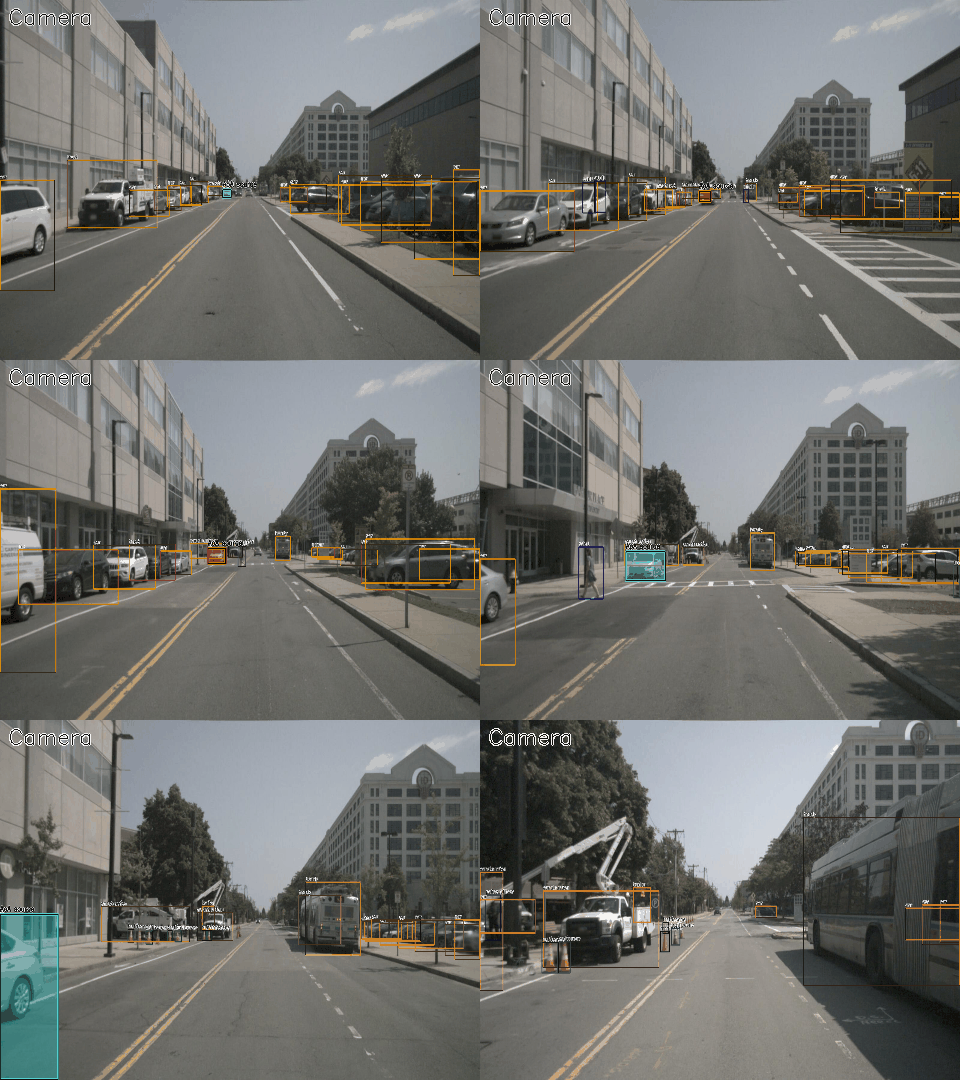
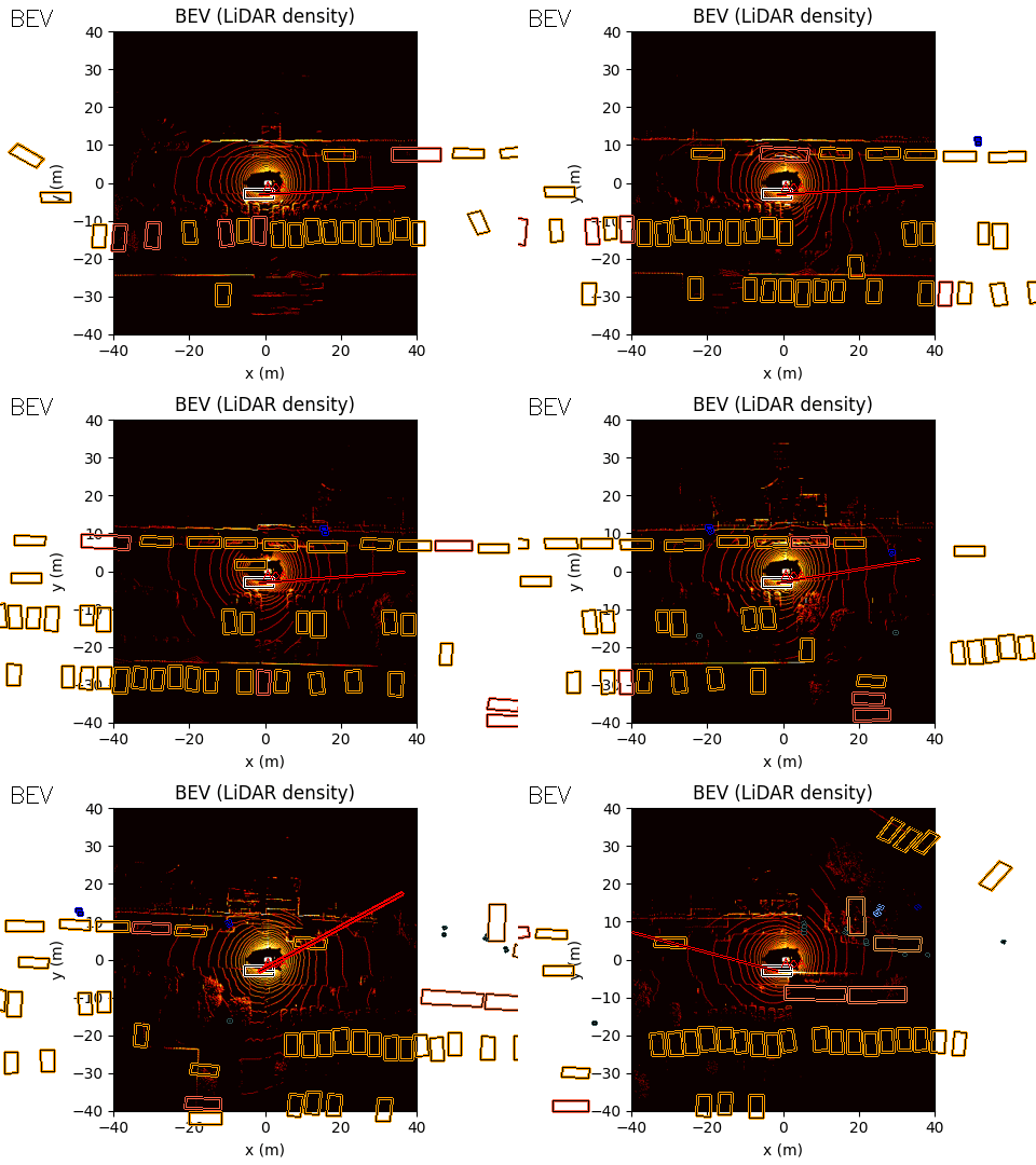
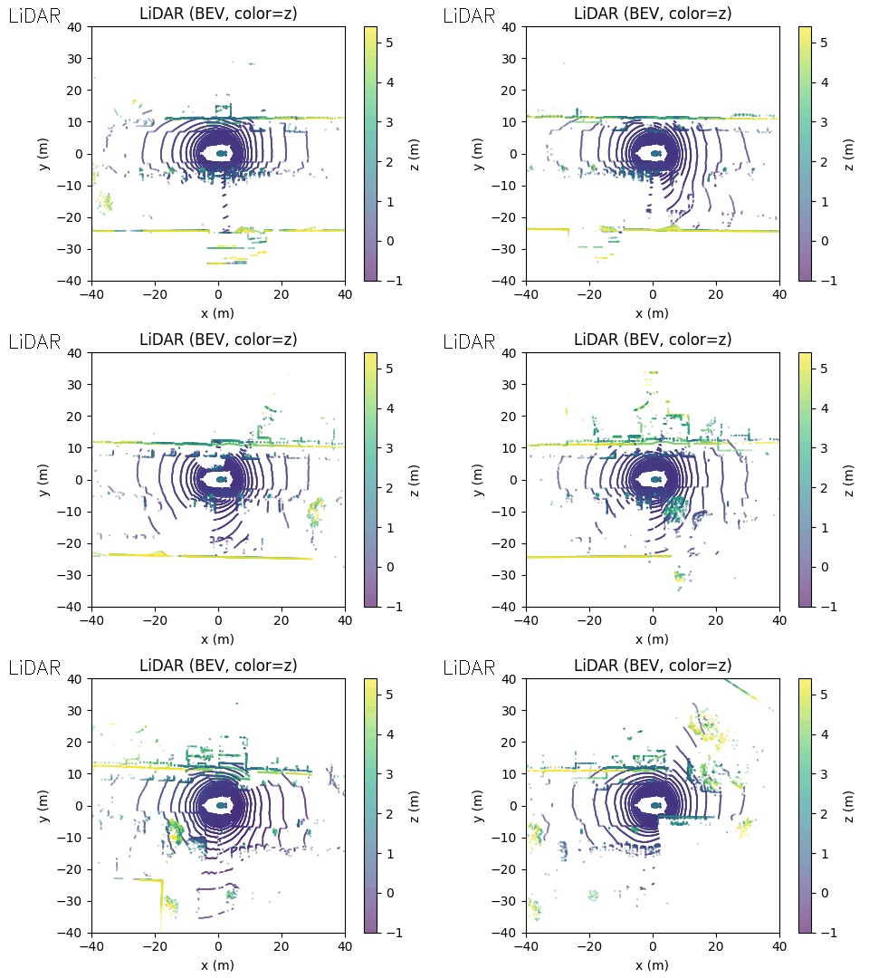
In the example scene below, the ego vehicle drives past a stationary car that is simulated to emit an emergency vehicle siren. The figure illustrates how the acoustic signal integrates with the rest of the perception stack.
On the left, we show the acoustic output tagged with an object ID from the real-time object detection system provided by the customer (likely based on a model such as YOLO).
In the centre, we show the BEV representation, where the estimated angle of arrival (AoA) from the microphone array is plotted as a ray originating from the ego vehicle. Because the clip is only six seconds long, the visualization shows a ray pointing in the direction of the detected emergency vehicle sound from the start of the sequence. In this case, the microphones detect the siren before the object enters the field of view of either the camera or the lidar.
Once the vision-based detector identifies the vehicle, the AoA estimate can be associated with that object, with small corrections applied if necessary to account for sensor alignment or localisation error.
On the right, we show the lidar point cloud for the same scene. In this example, the acoustic output is not annotated in the lidar view, although such a visualization is also possible.
Camera: Flashing red/cyan vehicle is emitting sound
BEV: Acoustic AoA Plotted
LiDAR
Implementation Considerations
The passive acoustic monitoring pipeline can be implemented efficiently on embedded automotive hardware. In our implementation, the audio processing pipeline, machine learning inference, and angle of arrival estimation were designed to run on a single MCU core. This includes signal preprocessing, spectrogram generation, neural network inference, and cross-correlation based localization.
The system was implemented on Renesas automotive controllers, specifically the RH850 microcontroller family. Audio input processing, AI target detection, and angle of arrival estimation ran on a single RH850 core alongside the A2B audio stack. In this configuration the full acoustic pipeline occupied roughly 300 KB of code space, even while running in a debug configuration and without aggressive optimization.
This relatively small footprint makes it feasible to deploy acoustic sensing alongside other perception tasks without requiring specialized hardware acceleration. On RH850 devices, significant CPU, flash, and RAM resources remain available for additional vehicle functions.
Microphone array configurations can also be adapted depending on coverage requirements. A four-microphone array provides approximately 180 degrees of coverage, while an eight-microphone configuration enables full 360 degree sensing around the vehicle.
In practice, the computational requirements depend on the complexity of the processing pipeline. Efficient PAM processing can run entirely on automotive-grade microcontrollers such as the RH850. Larger microphone arrays or more complex neural networks may benefit from more powerful automotive SoCs such as the Renesas R-Car platform. Regardless of the hardware platform, maintaining real-time processing is critical so that acoustic events can be incorporated into the perception pipeline with minimal latency.
Passive acoustic monitoring has shown significant potential but has not yet become standard in autonomous vehicle perception stacks. There are several challenges that limit its adoption:
Ambient noise and signal variability – urban environments are full of sounds that can mask sirens, horns, and other important cues.
Environmental acoustic complexity – reflections, occlusions, and vibrations from the vehicle itself make accurate localization difficult.
Automotive qualification and safety standards – microphones and processing hardware must meet rigorous requirements such as ISO 26262 and AEC-Q100, and survive extreme temperatures and vibrations.
Limited generalization of machine learning models – systems that perform well in controlled tests can struggle on highways, in multi-siren urban settings, or with unusual sound events.
No regulatory requirement – without a mandate from safety standards or OEMs, there is little commercial incentive to integrate acoustic sensing into production vehicles.
Despite these obstacles, acoustic sensing can still provide value when used as a complementary modality. Integrating sound cues through late fusion on top of camera and lidar tracks allows early warnings of approaching emergency vehicles or other hazards, even before they enter the field of view. In this way, the acoustic signal reinforces and augments traditional sensors, enhancing situational awareness without requiring a full redesign of the perception stack. Performance improvements were observed in EuroNACP obstructed view testing scenarios, demonstrating the practical benefit of including an acoustic modality in complex urban environments.
]]>
https://franciscormendes.com/2026/03/07/acoustic-sensor-fusion/2026-03-07T05:00:00.000ZExploring PAMVON, a passive acoustic monitoring system for emergency vehicle detection, and the challenges preventing its production adoption.Beyond Photons: Passive Acoustic Sensing for Autonomous Vehicles2026-04-18T15:56:33.449ZFrancisco Romaldo Fernandes MendesIntroduction
Sometimes it does seem like my blog is just increasingly complex applications of the Fourier Transform. In the previous post we applied the Fourier Transform to graphs, drawing connections between frequency (which is the usual Fourier transform) and properties of the graph. There is yet another interesting, if abstract, application of the Fourier transform that is used in Quantum computers. Somewhat surprisingly, it is called the “Quantum Fourier Transform”. More specifically, we will study how the Fourier Transform appears as a unitary linear operator acting on quantum states.
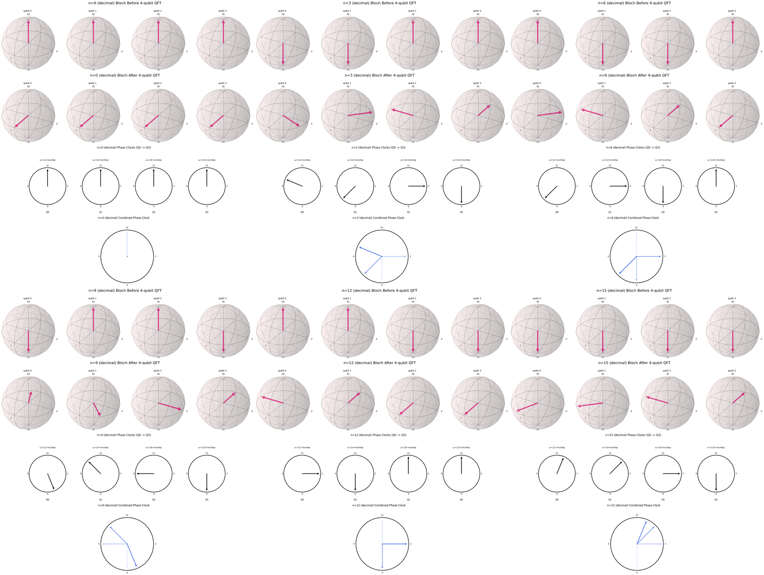
At the end of the day this is all just linear algebra, requiring no knowledge of actual quantum physics. Because the Quantum Fourier Transform can be somewhat mathematically abstract and also because the Fourier Transform is so easily visualized as a decomposition into various sines and cosines, I thought of coming up with a similar visualization for the Quantum Fourier Transform case (spoiler: it involves clocks).
Motivation
Before discussing in detail what the QFT is mathematically, it is useful to recap what the Fourier transform is in general. The Fourier transform is a way of transforming information from one domain to another domain. Why? Because certain operations become simpler in the transformed domain. For example, in classical signal processing, convolution of a signal (the mathematical definition of filtering) in the time domain corresponds to simple multiplication in the frequency domain.
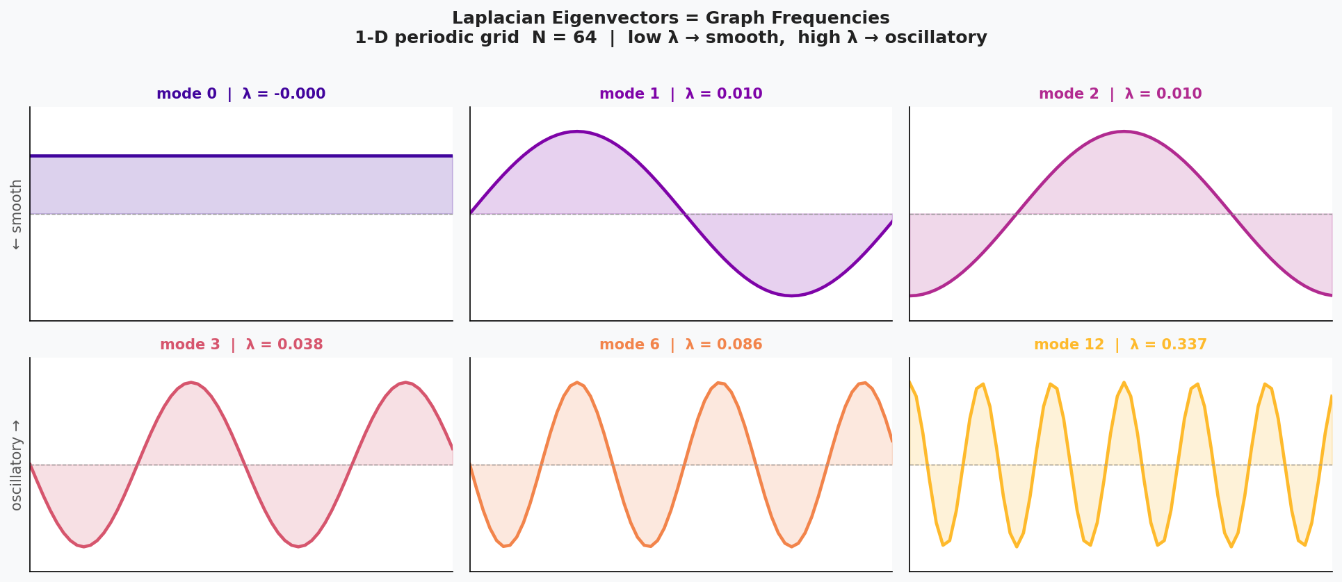
In the graph setting, we saw that potentially complex behaviors in the edge-node representation of the graph were far more mathematically tractable when looking at the “frequency” equivalent of the graph. Eigenvectors of the graph Laplacian isolate modes of variation: low-frequency components capture global structure, while high-frequency components capture local fluctuations.
Similarly, for the Quantum Fourier Transform, we move from a bit representation of a number to a cyclical or phase representation. In the computational basis, information is stored as binary digits, essentially a sequence of ON/OFF switches taking values in $\{0,1\}$.
In this form, the data is linear and rigid. Any underlying periodic structure is hidden inside the positional encoding. Phases, however, live on the circle and are inherently cyclical. If we want to detect periodicity or modular structure, it is more natural to encode information as rotations rather than switches.
The QFT therefore plays the same conceptual role as the classical Fourier transform: it changes coordinates to a representation in which the problem’s hidden structure becomes easier to manipulate.
I might do a post later on why this is true on so many different problems. But it is not true for some problems such as when you need convolution to learn a local filter.
Useful Intuition
One of the reasons the Fourier transform in its simplest form is so interesting is that it is so visual. In this blog post I will try to provide a nice visual explanation for the QFT. Essentially we want to draw a connection between the binary representation of a number and the cyclical nature of the QFT. Fortunately, there is a nice visual representation for a binary representation of a number on a computer, called a qubit. This representation of a number is called a qubit.
A Useful Visualization
]]>
https://franciscormendes.com/2026/02/28/quantum-fourier-transform/2026-02-28T05:00:00.000ZVisual guide to the Quantum Fourier Transform: from binary numbers and roots of unity to the QFT circuit, with comparisons to classical DFT and implications for Shor's algorithm.From Bits to Clocks: A Visual Intuition for the Quantum Fourier Transform2026-04-18T15:56:33.540ZFrancisco Romaldo Fernandes MendesIntroduction
I was recently invited back to the MA department at UChicago for a career conference. Sitting there, listening and speaking, I found myself asking a rather uncomfortable question:
How much of what we value in education is pure signaling? Is this still true in the age of AI?
It is perhaps an opportune moment to recap the signaling model of education. In labour markets with asymmetric information, employers cannot directly observe ability. In Michael Spence’s signaling model, education does not necessarily increase productivity; instead, it separates high-ability individuals from others because it is less costly for them to acquire. In this paradigm, education serves as a “signal” of ability.
I think AI has changed this status quo because the cost of acquiring education has reduced to the point that there is no cost differential between high-ability and low-ability individuals for a large number of courses. To be more specific, the cost of sending a signal of education is reduced to the point of being indistinguishable between both groups. The cost of actually educating oneself is likely still lower for high-ability individuals, it’s just that sending this signal is easier.
This essay is intended to answer some of the questions that I recieved at the conference, some of which are outlined below,
But what does “actually” educating oneself really mean?
What does it look like? Which classes should I take?
What should be the emphasis of my self-study?
How do I position myself best for the job market?
Beyond The Signal: So What Should I Study?
In the old (read: pre-AI) world where education was largely signaling, I think taking classes that superficially but with high probability signaled education, such as cloud skills, basic Python programming, and machine learning applications, were good enough. But in the new world, the cost of acquiring these skills is zero. Thus high-ability individuals need to seek out higher difficulty tasks that are relatively lower cost for them to acquire in order to send a strong signal. Mathematical maturity, comfort with abstraction, and disciplined reasoning are not signals in themselves; they are capabilities that affect what you can build, debug, or invent.
Thus class choices should reflect these core values:
Mathematical courses that emphasize the core mathematics that make up machine learning, such as linear algebra and differential equations
Looking under the hood of machine learning, focusing on the mathematical fundamentals of machine learning
Social sciences courses that challenge your world view and force you to think about what the world should look like (more on this below)
Good Intellectual Health
More important than ever, and not specific to tech jobs but just life in general, is maintaining good intellectual health.
Reading books both in your field and outside of it is now more important than perhaps in the world before AI. Using AI increases one’s distance from one’s self. One’s ideas and one’s thoughts are now further than ever from one’s own experience. Reading books and writing reduces this distance. Since idea generation and critical thinking depend so heavily not only on the final output but also on the process by which one reaches it, exercising this muscle is now more important than ever.
Maintaining good intellectual health, however, is almost entirely self-policed. There are very few reliable ways to monitor how much AI shapes one’s own work. What usually starts as submitting homework in a rush can escalate to generating entire essays using AI, the slope is truly slippery. One cannot afford to replace the cognitive effort that builds depth, originality, and judgment. Only you can decide if the level of AI use hampers your intellectual health, and only you can feel its effects.
Emphasizing the Social Sciences
The sciences are exceptionally good at helping us understand what the world is. As a result, advice about improving technical skills tends to be prescriptive and measurable. The social sciences operate differently. They help us think about what the world should look like. They force us to articulate assumptions about behaviour, incentives, norms, and institutions. The process of forming a view about what the world ought to be is central to intellectual health. It requires reflection, judgment, and an awareness of values, not just optimisation. Admittedly, this is difficult advice to give at a career conference for students focused purely on technical roles. The impact of studying sociology, psychology, or economics is harder to measure in a tech performance review. It doesn’t map cleanly onto a skills matrix. But it is no less important for that reason. The social sciences implicitly construct world models. Whether in sociology, psychology, or economics, they offer structured ways of thinking about how systems of people behave. That kind of world-building is essential for understanding where highly parameterised models, such as those produced in machine learning, actually live. Models do not operate in a vacuum; they operate within social and economic systems.
This becomes even clearer in business contexts. Firms operate with explicit views of what the world should look like, in terms of acquisition, churn, retention, revenue. Machine learning systems are deployed inside those normative visions. I admit there is something slightly distasteful about motivating the social sciences purely in terms of churn or revenue. It feels almost sacrilegious. But in practice, those incentives shape the environments in which technical systems are built. And if that were not the case, the audience at a career conference might be asking very different questions, comrade.
TL;DR;
The “sticker” value of UChicago’s education has held steady relative to other similar institutions. It might even have appreciated slightly. However, the absolute “sticker” value of education as a signal of ability in top schools (and indeed everywhere else) has gone down. Thus the onus is now on students to take courses that more appropriately signal their ability, not just in purely technical terms (such as mathematics, physics, machine learning) but also in critical thinking terms (such as expertise in the social sciences). The days of superficial knowledge that use model.fit(X) are over.
The UChicago brand will likely hold its value for years to come but it is not going to be enough. Even though the bar to have superficial knowledge is lowered thus muddying the difference between high and low skill individuals, the bar to have truly fundamental understanding of the sciences including (and perhaps especially) the social sciences is has never been higher.
]]>
https://franciscormendes.com/2026/02/20/ssd-career-conference/2026-02-20T05:00:00.000ZSpence's signaling model updated for AI: when the cost of educational signaling collapses to near-zero, what genuine intellectual skill looks like and how to build it.Signaling, Skills, and Intellectual Health in the Age of AI: Thoughts from UChicago Career Conference 20262026-04-18T15:56:33.615ZFrancisco Romaldo Fernandes Mendes
I did not spend my twenties reading Murakami, when it was all the vogue. Now, having read three works of his, I feel an upswell of opinions on his work and writing. We will explore some of the themes of Murakami as well as the cultural symbol that he has become. He was the kind of writer you are almost supposed to like as a young man.
Murakami seemed like the sort of writer you are supposed to like, especially in your twenties. Sadly, my twenties flew by rather quickly without so much as a glance at a Murakami novel. And there were several — part of Murakami’s appeal is how prolific he is across a variety of genres. Now in my, arguably still early, thirties I have read three novels of his: Kafka on the Shore, First Person Singular, and The Wind-Up Bird Chronicle. While my views on Murakami remain lukewarm at best, his writing certainly inspires deeper engagement with broader themes in society.
Writing
The English literary tradition has always been deeply rooted in the beauty of language; it is almost as if the words carrying the story must match the beauty of the story itself. The result can be complex, layered prose that oftentimes outlasts the literary work itself. Very often from the opening lines themselves, the classics sought to set the stage with beautiful prose.
“Call me Ishmael…”, “It was the best of times, it was the worst of times…”
Compare this with Murakami, whose writing proceeds forth incessantly in its banality. The words easily slide off the page as if narrated by a friend over the telephone. The words do not linger; they hurry off the page carrying their message with great efficacy. He does not, however, use this efficiency to drive more of the plot forward, choosing instead to match the banality of his prose with descriptions of the banalities of the human condition — eating, sleeping, and listening to music. It seems as if Murakami rejects the aestheticism of both the prose and the story. One cannot imagine Dickens devoting a paragraph to what the main character ate for breakfast.
One should not leave with the impression that the resulting writing is uninspired or insipid. On the contrary, the effect of his writing is a highly atmospheric narrative style that attenuates his trademark surrealistic elements. The banalities serve to obscure or highlight the passage of time, a critical element of his surrealistic themes. The reader is drawn into a different world, and very often drawn into a different supernatural world within that world.
A long-standing critique of English literature prior to Murakami was that it was almost inaccessible to people learning English for the first time. In my eyes this was largely a consequence of English speakers dominating English writing, whereas Murakami does not speak English as his first language. Nothing exemplifies this more than the fact that Murakami came upon his extraordinarily simple writing style by simply translating his English prose to Japanese and then back, thus losing all but its most essential elements. Literary essentialism, some (this author) would call it.
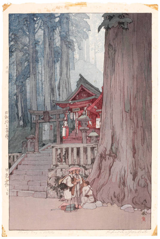
Nothing is happening here. The shrine stands. The snow falls. And yet — this is precisely the kind of scene Murakami would spend three pages on, and you would read every word of it. The atmosphere is the point; the banality is the vehicle. This is the closest image I can find to what it actually feels like to read him.
Eastern Storytelling
There is a tension between Eastern and Western storytelling, and this tension is apparent even in the differences in children’s stories. In Grimm’s fairy tales, for example, we have a clearly defined protagonist who must weather the odds, defeat the antagonist, and eventually prevails. In Eastern storytelling the beauty of the story is much more important than what the story means. Consider The Crane Wife, a well-known Japanese children’s story. A crane transforms into a beautiful woman; this beautiful woman proposes to a poor fisherman. The fisherman agrees, but the woman imposes one condition: he can never look at her when she is weeping. One day the fisherman looks at her while she weeps; he sees that she is a white crane. He leaves her. The story ends, rather abruptly. This ending is rather distressing, especially to Western audiences. Why does the story end? The ending is so sad — how can it end yet? What does this all mean? Beauty, I suppose, is the key to this difference. This is a beautiful story and the sadness is beautiful.
The moon reflects on the water. The islands sit in the dark. No story. No explanation. No moral. And it does not matter — the image is enough. This is what Eastern aesthetic beauty looks like when it works. Murakami is reaching for something like this. I am not always sure he grasps it.
I have the same visceral reaction to Murakami’s stories. I find myself asking at the end of every book:
But what does this all mean?
While I recognize that this cultural difference is at the heart of why people react negatively to Murakami’s writing, I find it hard to reconcile with the fact that Murakami’s writing forces you to do one of two things.
The first is to take the story literally. This involves taking every supernatural act, every bizarre event as literal and believing it. This is not hard — we do this to some degree with all works of fiction, from Tolkien to Kafka. We are (I am) willing to suspend disbelief. However, the stories take themselves seriously. In The Metamorphosis, while we are never offered an explanation for why Samsa is a monstrous insect, the reactions to him and his reactions to himself treat his metamorphosis as real. The story takes itself seriously and reconciles the apparent inexplicability of the metamorphosis as given. This is not the effect that Murakami’s writing has on me. His writing weakly evokes bizarre situations such as the insect; however, there are a great many such situations. The immoderation in the supernatural and the bizarre requires a much higher degree of suspension of disbelief, which makes it much harder for the reactions of other characters to be believable. It reminds me of the famous Christopher Nolan quote:
“It does not matter how believable the story is to you; the story must be believable to itself and its characters.”
It is this inviolable rule that is broken multiple times.
The second is to take the story as some kind of metaphor. Again, Kafka’s writing has this effect as well — we can think of the insect-like transformation of Gregor Samsa as a kind of moral corruption, stagnation, or emasculation. However, because Murakami uses characters, bizarre events, and other supernatural motifs so liberally, it is difficult for the metaphor to retain any coherent narrative structure, let alone a consistent representation of something else.
In both cases, it seems as if Murakami is willing to sacrifice coherence and linguistic beauty for some kind of narrative aesthetic. To me this sacrifice was not worth it, since there are far too many characters and motifs that seem to exist solely to move the plot along. Far too many characters are sacrificed on this imagined altar of aesthetic beauty. My objection does not arise out of a sense of wellbeing for these characters, but rather that they seem rather superficial — which leads naturally to my next criticism.
Superficiality
The main characters in Murakami’s books can be disappointingly without agency. They can seem as if they are carried away by the wave of the narrative. This matches Murakami’s style in his own words: he creates the characters first and then places them in a story. Almost like a simulation — this makes the storytelling easy.
Again, this could be the difference between Eastern and Western protagonists. I do not agree with this, however. I think Murakami’s characters are quite American in a modern way. The protagonist is like the main character in a pop culture film — hidden away, not a part of society. But then society needs him, or something happens to him, and he must act in the midst of it. In some strange way this superficiality matches the aesthetic of Murakami’s writing. In some ways, I consider Murakami to be a modern American author, as much as Paul Auster. To Murakami’s credit, I suspect this imitation might not be entirely unintentional. This imitation evokes the adoption of Western individualism by Japanese society — fairly thin, and without the corresponding import of Christian ethics. Murakami laments the lack of family connections in Japanese society.
Similarly, supporting characters exist only as reflections of the main character. In all the books that I read, I was not able to identify one single character that had anything remotely resembling a personality. Murakami writes a superficial main character and every other character exists to reflect that character back to himself. Bizarrely, Murakami’s novels feel two-dimensional — you are drawn into an atmospheric but ultimately flat world. Some things feel real, but the lack of dimension is apparent. It has to be said that this is appealing to some; others describe this as “dreamy”, “vague”, and “beautifully foggy”. It is likely that this flaw uniquely penetrates my intellectual armor more so than others.
I have many issues with the way women are written in Murakami’s novels. I will leave it at that.
Japanese Psyche
It is somewhat contradictory that Murakami is surprisingly modern, and almost comes across as an American writer in some sense. Yet the questions his books raise about Japanese identity — individualism imported wholesale from the West, the erosion of family and community — are distinctly Japanese concerns, and they are the more interesting for it.
Conclusion
I find myself, having now read three of his novels, in the rather uncomfortable position of a reluctant critic. Murakami is undeniably significant. He has done more for the global reach of Japanese literature than perhaps any other living author, and his ability to inhabit the borderlands between the real and the supernatural is a genuine literary achievement. His cultural impact is not nothing, as the young person in every bookshop clutching a copy of Norwegian Wood will attest.
But the books themselves leave me cold — not in a sterile sense. They are atmospheric, readable, and at times deeply evocative. I always emerge from them, however, without the feeling of having had a meaningful encounter with another human mind. The characters drift, the plots dissolve, and one is left with that same persistent question.
But what does this all mean?
I suspect that for his devoted readers, the answer is in the question itself. The asking is the point. The fog is the destination. I remain unconvinced, but I respect the fog.
Murakami’s world looks something like this — solid enough to walk through, obscured enough to never quite see the edges of. The fog does not owe you an explanation. I have made my peace with this, though not enough to enjoy it.
]]>
https://franciscormendes.com/2026/01/15/on-murakami/2026-01-15T05:00:00.000ZHaving now read three of his works — Kafka on the Shore, First Person Singular, and The Wind-Up Bird Chronicle — some lukewarm opinions on Murakami.On Murakami2026-05-21T15:56:02.542ZFrancisco Romaldo Fernandes MendesIntroduction
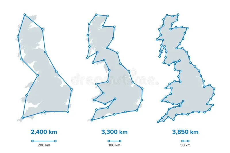
If you’ve ever come across the coastline paradox, you’ve probably seen the classic (and somewhat overused) image of the coastline of Britain. Recently, a friend asked me a question that felt like the 3D analogue of this paradox: What is the surface area of a city? More specifically, does a very hilly city have more surface area than a relatively flat one?
The answer, as it turns out, is more complicated than it first appears. My initial instinct was to treat this as the 3D version of the coastline paradox, and that idea sent me down a rabbit hole—one whose key insights form the basis of this blog post. Complete follow along notebook can be found here.
Here’s how the post is structured:
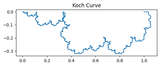
Visualizing the 2D coastline paradox using the Koch curve, a well-known fractal curve.
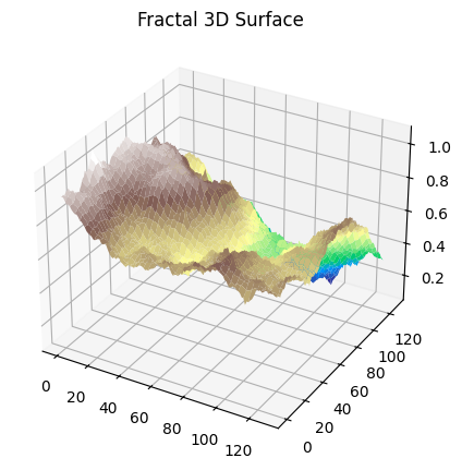
Extending this to the 3D case by visualizing the surface area paradox with a fractal terrain.
Applying these ideas to real-world GIS data to verify the paradox in practice.
Exploring the concept of dimension.
Point 4 turned out to be particularly enlightening. In researching this post, I realized that the way we commonly think about “dimension”—1D, 2D, 3D—is not mathematically rigorous. The coastline paradox and its 3D surface area counterpart only exist because our intuitive notion of dimension is incomplete. In fact, dimensions can be fractional, and by using the results from sections 1, 2, and 3, we can actually measure them and gain a deeper understanding of the geometry underlying these paradoxes.
2D Coastline Paradox
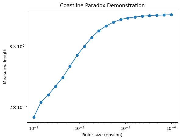
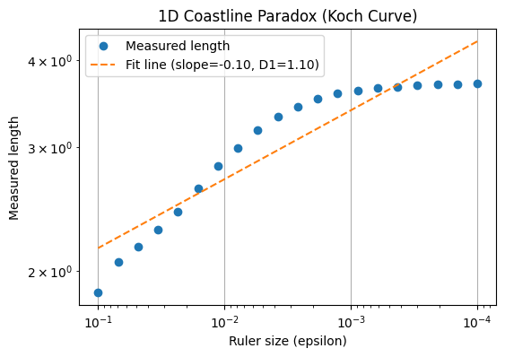
The figure above illustrates the coastline paradox using a Koch curve, a classic fractal curve. As the ruler size decreases, the measured length of the curve increases dramatically, highlighting that the “true” length of a jagged, self-similar shape is not well-defined. In the top plot, we visualise the Koch curve after six iterations, showing its intricate zig-zag pattern. The bottom plot demonstrates the paradox quantitatively: on a log–log scale, smaller ruler sizes (on the right) capture finer details, resulting in a rapidly increasing measured length. This simple experiment illustrates why fractal curves require a scale-invariant descriptor—the Minkowski or box-counting dimension—to characterise their complexity, rather than relying on a single length measurement.
The figures above illustrate the coastline paradox using a Koch curve, a classic fractal curve. As the ruler size decreases, the measured length of the curve increases dramatically, highlighting that the “true” length of a jagged, self-similar shape is not well-defined. In the top plot, we visualise the Koch curve after six iterations, showing its intricate zig-zag pattern. The bottom plot demonstrates the paradox quantitatively: on a log–log scale, smaller ruler sizes (on the right) capture finer details, resulting in a rapidly increasing measured length. This simple experiment illustrates why fractal curves require a scale-invariant descriptor—the Minkowski or box-counting dimension—to characterise their complexity, rather than relying on a single length measurement.
Mathematical Proof
Consider a jagged curve (e.g., a coastline) in 2D, and let $L(\varepsilon)$ denote the measured length using a ruler of size $\varepsilon$.
Divide the curve into segments of length $\varepsilon$. Let $N(\varepsilon)$ be the number of segments required to cover the curve:
If the curve is smooth: $D = 1$, then $L(\varepsilon) \sim \varepsilon^{0} = \text{constant}$.
If the curve is fractal: $D > 1$, then $L(\varepsilon) \to \infty$ as $\varepsilon \to 0$.
This demonstrates the paradox: the measured length depends on the ruler size, and only the fractal dimension $D$ provides a scale-invariant measure of the curve’s complexity.
On a log–log plot of $L(\varepsilon)$ vs $\varepsilon$, the slope is $1-D$.
This allows us to characterise the roughness of the curve quantitatively.
3D Coastline Paradox
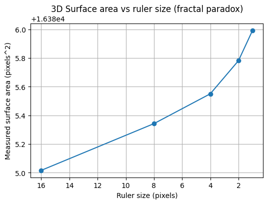
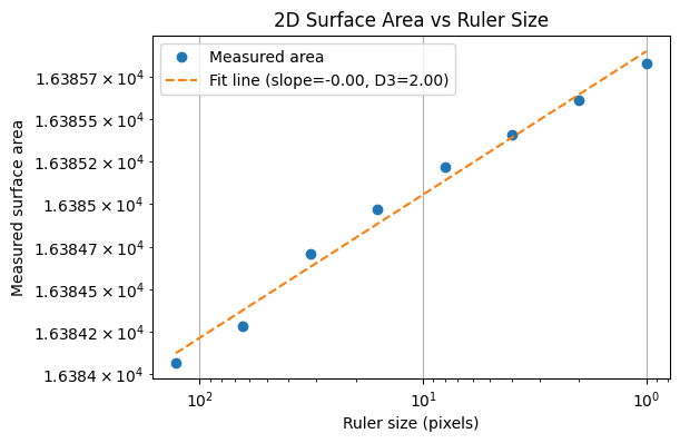
The figure below demonstrates the geographical area paradox, the 3D analogue of the coastline paradox. Here, we measure the surface area of a fractal terrain generated using the diamond-square algorithm. As the size of the measurement “ruler” (square grid) decreases, the measured surface area increases, revealing more of the fine-scale roughness of the terrain. Just as the length of a fractal curve diverges with smaller ruler sizes, the area of a fractal surface grows without bound. This shows that for rough surfaces, the conventional notion of area is ill-defined at very small scales. Instead, the fractal dimension of the surface provides a single, scale-invariant number that quantifies the complexity of the terrain.
Mathematical Formulation of the 3D Surface Paradox
Consider a 3D surface $z = f(x,y)$ defined over a 2D domain. Let $A(\varepsilon)$ denote the measured surface area using a square ruler of side $\varepsilon$.
Divide the plane into a grid of squares of side (\varepsilon). Let $N(\varepsilon)$ be the number of squares required to cover the surface (or, equivalently, the number of boxes intersecting the surface in 3D):
On a log–log plot of $A(\varepsilon)$ vs $\varepsilon$, the slope is $2$D.
This provides a scale-invariant measure of the surface’s roughness analogous to the 2D case but in two dimensions.
Telegraph Hill
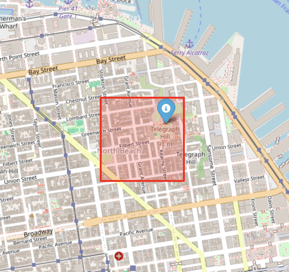
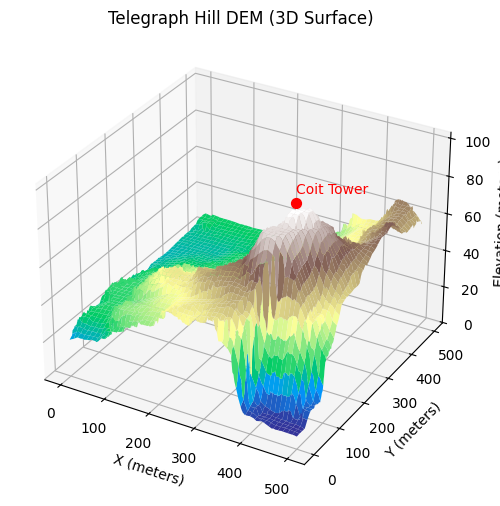
Up to this point, we have illustrated the coastline (or geographical area) paradox using a simulated fractal surface. While this is useful for building intuition, it is ultimately a controlled toy example. In this section, we replace the synthetic terrain with real elevation data from Telegraph Hill in San Francisco. Extracting and preparing this data turned out to be an ordeal in its own right—one that probably deserves a dedicated blog post. There is something uniquely satisfying about working with GIS data: every raster, projection, and coordinate transform is a walking demonstration of linear algebra in the wild. But I digress. With the elevation data in hand, we can now repeat the same multi-scale measurement exercise and observe the coastline paradox emerge not from a mathematical construction, but from an actual piece of geography.
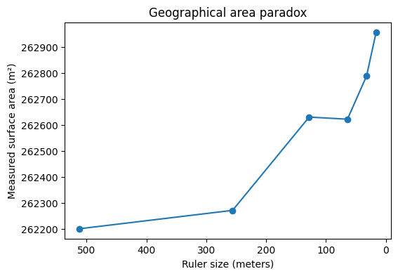
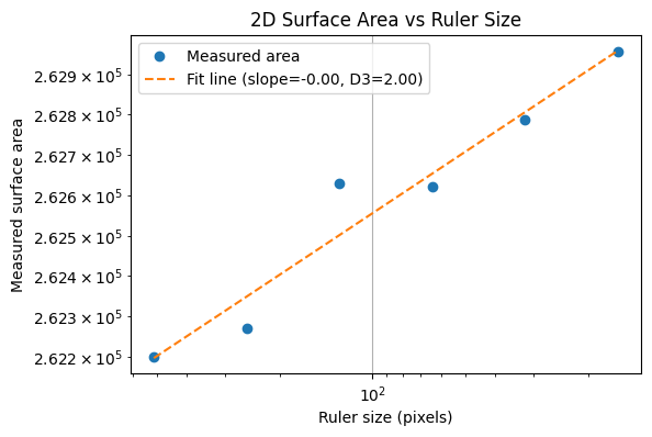
To illustrate the coastline paradox in a real geographical setting, we estimate the surface area of Telegraph Hill using progressively smaller “rulers.” In the code above, the terrain is measured with square rulers of 256, 128, 64, and 32 meters, and the total surface area is recomputed at each scale. As the ruler size decreases, the measured area systematically increases. This is not because the hill is physically changing, but because finer rulers capture more of the terrain’s small-scale roughness—minor ridges, gullies, and local slope variations that are invisible at coarser resolutions. The resulting curve demonstrates the geographical area paradox: for a rough, fractal-like surface, area is not a single well-defined number, but a scale-dependent quantity. What remains invariant across scales is not the measured area itself, but the rate at which it grows as the ruler size shrinks—an idea formalised by the surface’s fractal dimension.
Fractional Dimensions
So far, we have seen how measured length or surface area depends on the ruler size: smaller rulers reveal more detail, producing larger measured values. The key insight of fractal geometry is that this scale-dependence can be quantified by a fractional, scale-invariant dimension, also called the Minkowski–Bouligand dimension.
2D Case: Koch Curve
For a fractal curve, the measured length (L(\varepsilon)) scales with ruler size (\varepsilon) as:
$$L(\varepsilon) \sim \varepsilon^{1-D_1} = 1.1$$
where $D_1$ is the fractal dimension of the curve. By plotting $\log L(\varepsilon)$ versus $\log \varepsilon$, the slope of the line gives $1-D_1$, from which we can solve for $D_1$. For the Koch curve, this yields $D_1 \approx 1.1$ (theoretically this is $1.26$), reflecting that the curve is “rougher than a line” but does not fill a plane.
3D Case: Simulated Fractal Surface
For a fractal surface, the measured area $A(\varepsilon)$ scales with ruler size $\varepsilon$ as:
where (D_2) is the surface’s fractal dimension (with $2 < D_2 < 3$). A log–log plot of $A(\varepsilon)$ versus $\varepsilon$ gives a slope of $2-D_2$, allowing us to solve for $D_2$. In practice, simulated terrains often have $D_2 \approx 2.3{-}2.5$, meaning the surface is rougher than a plane but still does not fill 3D space.
Real-World Case: Telegraph Hill
Finally, we can apply the same method to elevation data from Telegraph Hill. Using square rulers of decreasing size, we measure the terrain’s surface area at each scale. A log–log plot of measured area versus ruler size produces a slope that corresponds to $2-D_{TH}$.
The resulting fractional dimension (D_{TH}) captures the true roughness of the hill, providing a quantitative, scale-invariant measure of the terrain’s complexity. Just like with the Koch curve or the simulated fractal surface, the hill exhibits a dimension that is between its topological dimension (2) and the embedding dimension (3), revealing the fractal nature of real-world landscapes.
The Fractal Boundary of Trainability
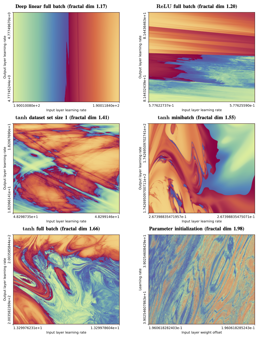
The most interesting region of hyperparameter space is not where training clearly succeeds or clearly fails, but the boundary between the two. This is where learning rates are just stable enough, regularisation is just sufficient, and optimisation teeters on the edge of divergence.
When we zoom into this boundary between convergent (blue) and divergent (red) training regimes, something remarkable happens: structure appears at every scale. Regions that look smooth at coarse resolution reveal increasingly intricate patterns as we zoom in. No matter how closely we examine it, the boundary never simplifies.
In this sense, the boundary of neural network trainability behaves like a fractal. Just as with coastlines or rough surfaces, the distinction between “trainable” and “untrainable” depends on the scale at which we probe it — a reminder that even optimisation lives in a world of fractional geometry.
Scale dependent kinematics: spacetime extension
One intriguing extension is to imagine motion along a fractal path, where the effective distance depends on scale. If $L(\varepsilon) \sim \varepsilon^{1-D}$ is the measured length at scale $\varepsilon$, then a “scale-dependent velocity” $v(\varepsilon)$ could be written as:
For a particle moving in a fractal spacetime geometry, this hints at scale-dependent kinematics, where the observed velocity changes with the measurement resolution, connecting fractal dimension $D$ with the local structure of spacetime.
Conclusions and Final Thoughts
Through this exploration, we have seen how the coastline paradox extends naturally from 2D curves to 3D surfaces, and how it manifests in real-world terrain like Telegraph Hill. Starting with the Koch curve, we visualized the fundamental idea that measured length depends on the scale of measurement. Extending this to 3D, we saw that the surface area of a rough, fractal-like terrain increases as the measurement resolution becomes finer—a phenomenon we’ve called the geographical area paradox.
Applying the same principles to actual GIS data confirmed that this is not just a theoretical curiosity: hilly cities truly do have “more surface” at finer scales, and the apparent area depends on how finely it is measured.
Finally, this journey highlighted the importance of fractional dimensions. Traditional notions of dimension—1D, 2D, 3D—are insufficient to capture the complexity of fractal structures. By calculating Minkowski–Bouligand dimensions from 1D curves, 2D surfaces, and real-world elevation data, we gained a quantitative, scale-invariant measure of roughness.
In the end, the coastline paradox is more than a curiosity: it offers a window into the hidden complexity of the world, from jagged coastlines to hilly terrain, and pushes us to rethink the conventional notion of integer dimensions. Indeed, questioning our intuition about dimensions may be essential for a deeper understanding of concepts like velocity, especially when the underlying physical paths we traverse may be inherently fractal.
]]>
https://franciscormendes.com/2025/12/16/3d-coastline-paradox/2025-12-16T05:00:00.000ZDoes a hilly city have more surface area than a flat one? The 3D coastline paradox explored via fractal dimension, Hausdorff measure, and a Python notebook applied to Telegraph Hill.Telegraph Hill and the Coastline Paradox: Measuring a City in Fractional Dimensions2026-04-18T15:56:33.443ZFrancisco Romaldo Fernandes MendesIntroduction
Convolution sits at the heart of modern machine learning—especially convolutional neural networks (CNNs)—yet the underlying mathematics is often hidden behind highly optimised implementations in PyTorch, TensorFlow, and other frameworks. As a result, many of the properties that make convolution such a powerful building block for deep learning become obscured, particularly when we try to reason about model behaviour or debug a failing architecture.
If you know the convolution theorem, a natural question arises:
Why don’t CNNs simply compute a Fourier transform of the input and kernel, multiply them in the frequency domain, and invert the result? Wouldn’t that be simpler and faster?
This blog post addresses exactly that question. We will see that:
FFT-based convolution is not local. In the Fourier domain every coefficient depends on every input pixel. This destroys the locality structure that CNNs rely on to learn hierarchical, spatially meaningful features. As a result, it breaks the very inductive bias that makes CNNs effective.
FFT-based convolution is not computationally cheaper in neural networks. Although FFTs are asymptotically efficient, they must be recomputed on every forward and backward pass—and the cost of repeatedly transforming inputs, kernels, and gradients outweighs any benefit from spectral multiplication.
By the end of this post, we’ll have a clear, explicit comparison—both in matrix form and via backpropagation—showing why CNNs deliberately perform convolution in the spatial domain. Any practioner of signal processing should also be interested in knowing when the “locality” property is useful and when it is not!
1-D Convolution
Let us start with the most basic form of convolution, the 1D convolution. In this case you have a filter (which is nothing but a sequence of numbers) that you want to multiply with your signal in order to produce another signal which is hopefully more interesting to you. For example, in your headphones, you want to multiply a set of numbers with the music signal such that the resulting signal is more music than the wailing baby 1 row behind you.
1 2 3 4 5 6 7 8 9 10 11 12 13 14 15
import numpy as np
defconv1d_direct(x, h): nx, nh = len(x), len(h) y = np.zeros(nx+nh-1) for n inrange(len(y)): for m inrange(nx): k = n - m if0 <= k < nh: y[n] += x[m] * h[k] return y
x = np.array([1.,2.,0.,-1.]) # this is the signal of music + baby wailing h = np.array([0.5,1.,0.5]) # this is a filter that when multiplied with x makes it more music conv1d_direct(x,h)
Convolution Theorem
This brings us to the convolution theorem wherein we can prove that the process of convolution i.e. multiplying window-wise h and x is mathematically equivalent to a simple multiplication between the fft of h and the fft of x.
1 2 3 4 5 6 7 8 9
defconv_via_fft(x,h): N = len(x)+len(h)-1 X = np.fft.rfft(x,n=N) H = np.fft.rfft(h,n=N) return np.fft.irfft(X*H,n=N)
Just like before before we will convolve a 2D filter with a 2D signal in the spatial domain. We will then, try to do it using the FFT. We will verify that the convolution theorem does indeed work in the 2D space as well.
1 2 3 4 5 6 7 8 9 10 11 12 13 14 15 16
defconv2d_direct(img, ker): ih, iw = img.shape kh, kw = ker.shape out = np.zeros((ih+kh-1, iw+kw-1)) for i inrange(out.shape[0]): for j inrange(out.shape[1]): for m inrange(ih): for n inrange(iw): km, kn = i-m, j-n if0 <= km < kh and0 <= kn < kw: out[i,j] += img[m,n] * ker[km,kn] return out
img = np.array([[0,0,0,0],[0,1,2,0],[0,3,4,0],[0,0,0,0]]) ker = np.array([[1,2,1],[2,4,2],[1,2,1]])/16 conv2d_direct(img,ker)
Convolution Theorem 2D
In a similar way to the 1D case instead of windowing and multiplying, we can take the fft of the signal and the kernel and simply multiply.
In a neural network, convolution is used to generate feature maps that feed into the next layer. At first glance, the convolution theorem suggests a tempting shortcut: instead of sliding a kernel spatially, we could transform both the image and kernel into the frequency domain, multiply them element-wise, and transform the result back. The output would be mathematically equivalent—so why not do this inside CNNs?
It turns out there are two fundamental reasons:
Neural networks care about more than just the output—they care about how the output is produced. During backpropagation, each filter weight is updated using gradients derived from local spatial features. This locality enables CNNs to learn hierarchies of edges, textures, shapes, and patterns. In the Fourier domain, however, gradients flow through global Fourier coefficients. Every frequency component depends on every pixel, so the update for a single weight depends on the entire image. This destroys the spatial locality that CNNs rely on and eliminates the inductive bias that makes them effective.
The FFT is not “simpler” computationally for neural networks. While FFTs are efficient in isolation, a CNN would need to repeatedly compute forward FFTs, spectral multiplications, and inverse FFTs—not just for the forward pass, but also for backpropagation. When you count actual multiplications and transforms, the FFT approach is often more expensive, especially for small kernels (e.g., 3×3, 5×5), which dominate modern architectures.
In short: CNNs avoid the Fourier domain because it removes locality and adds computational overhead—both of which undermine the very reasons convolution works so well in deep learning.
2D Spatial Convolution as a Matrix Multiply
For our next trick we will show the exact way in which your hardware actually computes convolutions. Spoiler: it will be some kind of matrix multiplication. This is quite different from the way convolution is taught in the classroom where you usually convolve with a patch of pixels in the spatial domain and roll the kernel onto the next patch nearby. In reality, this whole process is just represented as one huge matrix multiply. It is very important to think about convolution in this way, as it makes approaching complex questions easier. Since looping over pixels is not a coherent mathematical approach whose complexity is easy to compute. Once it is expressed as a matrix multiply between to matrices we can directly use a formula to compute complexity. More importantly, GPUs work fast precisely because they can parallelize this matrix multiply (as opposed to parallizing various kinds of for-loop structures).
In this section, $X$ denotes the input image. It’s worth noting that most deep-learning libraries treat the 2D and 1D cases in essentially the same way: the very first step is to reshape the image into a long vector, commonly written as $\mathrm{vec}(X)$. This operation—often implemented as im2col in the source code—unrolls local patches of the image so that convolution can be expressed as a matrix–vector multiplication.
Eventually these two values will be numerically the same! We know this from the convolution theorem. In the next section we will see that the contributing values matter to the gradient back propagation and that is where the two approaches will differ.
Spatial convolution is cheaper for small kernels, which is why CNNs prefer it.
FFT becomes advantageous only for very large kernels or very large images.
TL;DR
Spatial convolution is efficient for small kernels and preserves locality which is crucial for CNNs to learn hierarchies.
FFT convolution has global interactions, destroys the local inductive bias, and is only computationally advantageous for very large kernels.
Conclusion
We have seen that spatial convolution is not only computationally more efficient but also better suited to capturing the hierarchical structure inherent in most images. For instance, a face detection algorithm may rely on local patterns such as the triangle formed by the eyes and the nose. A kernel that focuses specifically on this local arrangement is highly effective because it preserves locality.
Conversely, in domains like recommendation systems, where data may be represented as a sparse matrix of product–user interactions, capturing global patterns can be more important. Here, the “local” interactions often correspond to users with strong connections, whereas broader, global patterns reveal trends across the entire system. In such contexts, FFT-based approaches—or methods that leverage global connectivity, like graph convolutional networks—can be more appropriate.
This contrast explains why spatial CNNs excel in image-based tasks, while GCNs or FFT-based methods are more suitable for graphs representing global interactions, such as those between users and products.
“A Friendly Introduction to Graph Neural Networks” (Stanford) – Excellent intuition about GCNs and why they differ from CNNs. https://web.stanford.edu/class/cs224w/
]]>
https://franciscormendes.com/2025/12/06/convolution/2025-12-06T05:00:00.000ZA unified treatment of 1D signal convolution, 2D image convolution via the convolution theorem, and graph convolution as a spectral operation on the normalized Laplacian.Locality, Learning, and the FFT: Why CNNs Avoid the Fourier Domain2026-04-18T15:56:33.518ZFrancisco Romaldo Fernandes MendesIntroduction
This is Part 2 of the series. In Part 1 we derived the Graph Fourier Transform from the Laplacian eigenbasis and built up the one-layer Spectral GCN formulation. Here we put it to work.
foundations.ipynb — mathematical derivations from DFT to irregular graphs
Application of Spectral GCN: Heat Propagation
In this section, we investigate a simple setting where a Spectral Graph Convolutional Network (GCN) performs surprisingly well: predicting heat diffusion across a toroidal mesh. Although the spectral approach is elegant and effective in the right circumstances, it also highlights several structural limitations inherent to spectral methods.
Graph Model of Heat Propagation
When we zoom into a small patch of the torus and add the connecting edges, the mesh suddenly looks like a familiar graph. This makes the role of the graph Laplacian immediately intuitive.
We zoom in on the hottest point on the mesh and plot it as a graph by explicitly showing edges.
We simulate heat diffusion on the graph using the discrete heat equation:
$$\frac{dx}{dt} = -L x$$
where $x \in \mathbb{R}^N$ is the heat at each node and $L$ is the graph Laplacian. Starting from two random vertices with initial heat, we update the heat iteratively using a simple forward Euler scheme:
$$x_{t+1} = x_t - \alpha L x_t$$
storing the state at each timestep to visualize how heat spreads across the mesh. Low-frequency modes of $L$ correspond to smooth, global patterns of heat, while high-frequency modes produce rapid, local variations.
The wraparound plot below shows this dramatically: starting from a single point source, the heat arc expands symmetrically around the ring until it meets itself on the far side.
Graph Fourier Transform of Heat Propagation
In order to get intuition for how the Fourier transform behaves on a graph, consider the distribution of heat on the graph surface.
The heat on the graph is represented by a real number for each node (temperature or heat energy in joules), so the signal is a vector $$x \in \mathbb{R}^{N},$$ where $N$ is the number of nodes.
If there are $N$ nodes in the graph the (combinatorial or normalized) Laplacian is an $N\times N$ matrix $$L \in \mathbb{R}^{N\times N}$$.
We use the eigendecomposition of the Laplacian to move between the vertex domain and the spectral (frequency) domain: $$L = U \Lambda U^{\top}, \qquad\Lambda = \operatorname{diag}(\lambda_1,\ldots,\lambda_N), \qquadU = [U_1\; U_2\; \cdots\; U_N],$$ with the eigenvalues ordered $0=\lambda_1 \le \lambda_2 \le \cdots \le \lambda_N$. The graph Fourier transform (GFT) and inverse GFT are $$\widehat{x} = U^{\top} x, \qquad x = U \widehat{x}$$.
To visualise single-frequency modes we simply pick individual eigenvectors $U_k$: $$\text{low-frequency mode: } x_{\text{low}} = U_{k_{\text{low}}}, \qquad\text{high-frequency mode: } x_{\text{high}} = U_{k_{\text{high}}},$$ where a natural choice is $k_{\text{low}}=2$ (the first nontrivial eigenvector) and $k_{\text{high}}=N$ (one of the largest-eigenvalue modes). Each vector $U_k$ assigns one scalar value to every vertex; plotting those values on the torus surface gives the heat-colour visualisation.
Practical steps used to create the figure
Build a uniform torus mesh and assemble adjacency and Laplacian $L$.
Compute the eigendecomposition $L=U\Lambda U^\top$ (for small / moderate meshes) or compute a selection of eigenpairs (Lanczos) for large meshes.
Select a low-frequency eigenvector $U_{k_{\text{low}}}$ and a high-frequency eigenvector $U_{k_{\text{high}}}$.
[Optional; not done here; to show smaller values in absolute terms]Normalize each eigenvector for display: $$\tilde{x} = \frac{x - \min(x)}{\max(x)-\min(x)} \quad\text{or}\quad \tilde{x} = \frac{x}{\max(|x|)},$$ so colours are comparable across panels.
Render the torus surface and colour each vertex by the value $\tilde{x}$ using a diverging colormap (e.g. heat) and add a colourbar showing the mapping from value to colour.
Interpreting the GFT on the torus
Low-frequency mode. The plotted heat corresponds to $U_{k_{\text{low}}}$ (small eigenvalue). The signal varies smoothly over the torus: neighbouring vertices have similar values, representing broad, global patterns of heat.
High-frequency mode. The plotted heat corresponds to $U_{k_{\text{high}}}$ (large eigenvalue). The signal alternates rapidly across nearby vertices, producing fine-scale oscillations around the torus that represent high-frequency, localised variations.
Spectral intuition
Recall, we expressed discrete heat propagation on a graph as,
$$x_{t+1} = (I - \alpha L) x_t$$
where $L$ is the graph Laplacian and $\alpha$ is a small step size.
Using the eigendecomposition of $L$,
$$L = U \Lambda U^\top,$$
we can rewrite the propagation as
$$x_{t+1} = \big(I - \alpha U \Lambda U^\top\big) x_t = U (I - \alpha \Lambda) U^\top x_t.$$
Comparing with the spectral graph filtering form,
$$x_{t+1} = U g(\Lambda) U^\top x_t,$$
we can identify the corresponding filter as
$$g(\Lambda) \equiv I - \alpha \Lambda.$$
Applying a spectral filter $g(\Lambda)$ to a heat signal $x$ acts by scaling each mode:
$$x_{\text{filtered}} = U g(\Lambda) U^\top x$$
so a low-pass filter suppresses the high-frequency panel patterns and produces smoother heat distributions, while a high-pass filter accentuates the oscillatory features visible in the high-frequency panel.
The Heat Kernel: The Analytically Correct Filter
One particularly revealing special case: the heat equation $\frac{dx}{dt} = -Lx$ has a closed-form solution. Starting from initial condition $x(0)$ and evolving for time $t$:
This means the exact spectral filter for heat diffusion at time $t$ is the heat kernel:
$$h(\lambda, t) = e^{-\lambda \cdot t}.$$
Smooth modes (small $\lambda$) survive nearly unchanged; oscillatory modes (large $\lambda$) are exponentially suppressed. In code this is a single line:
This provides a physics-informed baseline: after training on heat-diffusion data, the learned weights $\theta$ should approximately recover this exponential shape. Heat diffusion is therefore an ideal test case for spectral GCNs—the ground-truth spectral filter has a known closed form, so we can verify that the network has learned something physically meaningful rather than a coincidental fit.
Neural Network To Learn $g_{\theta}(\Lambda)$
We can write a spectral graph convolution / filter with learnable parameters $\theta$ as
$$x_{t+1} = U g_\theta(\Lambda) U^\top x_t,$$
where $U$ is the eigenvector matrix of the Laplacian, $\Lambda$ is the diagonal eigenvalue matrix, and $g_\theta(\Lambda)$ is a diagonal matrix of learnable weights acting on each eigenmode.
This makes it explicit that each column vector $U_i$ (the $i$-th eigenvector) is scaled by the learnable weight $\theta_i$ in the spectral domain, and then transformed back to the original node space via $U$ to produce the predicted signal $x_{t+1}$.
PyTorch Implementation
The three core operations—GFT, elementwise filtering, and inverse GFT—translate directly to PyTorch matrix operations (from graph_fourier.py):
The graph Laplacian is assembled from the mesh topology in build_graph.py. Each triangular face contributes three undirected edges, self-loops are added for stability, and the degree-normalised form is computed:
1 2 3 4 5 6 7 8 9 10 11 12 13 14
defcreate_adjacency_matrix(mesh): vertices, faces = mesh.vertices, mesh.faces num_nodes = len(vertices) adj = np.zeros((num_nodes, num_nodes)) for face in faces: for i inrange(3): for j inrange(i + 1, 3): adj[face[i], face[j]] = 1 adj[face[j], face[i]] = 1 adj = torch.tensor(adj, dtype=torch.float32) + torch.eye(num_nodes) deg = adj.sum(dim=1) D_inv_sqrt = torch.diag(1.0 / torch.sqrt(deg)) L = torch.eye(num_nodes) - D_inv_sqrt @ adj @ D_inv_sqrt return adj, L
Why Use A Neural Network?
Two motivating examples illustrate the practical usefulness of such a model:
Partial Observations from Sensors In many real-world systems, heat or pressure sensors are only available at a small subset of points. The experiment uses 750 sensors placed on the torus using farthest-point sampling (FPS)—an algorithm that greedily picks each next sensor as the vertex farthest from all already-chosen sensors, ensuring uniform coverage of the surface rather than random clustering:
All non-sensor nodes are zeroed during training over 40 timesteps of diffusion (step size $\alpha = 0.4$). We train the Spectral GCN using only these sparse observations, yet the learned model reconstructs and predicts the heat field across all vertices on the mesh—effectively turning sparse sensor readings into a full-field prediction.
Generalization to a New Geometry One might hope that a model trained on one torus could be applied to a slightly different torus. Unfortunately, this is generally not possible in the GCN setting. The eigenvectors of the Laplacian form the coordinate system in which the model operates, and even small geometric changes produce different Laplacian spectra. As a result, the learned spectral filters are not transferable across meshes. This is a fundamental drawback of spectral GCNs. However, we shall see that the GCN framework inspires frameworks that do not suffer from this drawback.
Stability Issues And Normalization
While the Spectral GCN learns the qualitative behaviour of heat diffusion, raw training often leads to unstable predictions. After several steps, the overall temperature of the mesh may drift upward or downward, even though heat diffusion is energy-conserving. This is because the neural network makes predictions locally without obeying the laws of physics such as the law of conservation of energy. Which is why our predictions are on average “hotter” than the actual.
Two practical fixes alleviate this:
Eigenvalue Normalization. Applying a sigmoid or similar squashing function to the learned spectral filter ensures that each frequency component is damped in a physically plausible range. This prevents the model from amplifying high-frequency modes, which would otherwise cause heat values to explode.
Energy Conservation. After each predicted step, the total heat can be renormalized to match the physical energy of the system. This ensures that although the shape of the prediction is learned by the model, the magnitude remains consistent with diffusion dynamics. Empirically, this correction dramatically improves long-horizon stability.
Training Results
Training the SpectralGCN for 300 epochs with the Adam optimizer on 40 diffusion steps yields rapid convergence:
Epoch
MSE Loss
0
0.000352
50
0.000031
100
0.000017
150–300
≈ 0.000015
The model achieves roughly a 10× loss reduction in the first 50 epochs, then plateaus near $1.5 \times 10^{-5}$. The steep initial descent reflects the fact that most heat-diffusion structure is captured by the lowest few eigenmodes — the tail of the training curve squeezes out residual error from higher-frequency components.
Overall, the Spectral GCN provides a compact and interpretable model for heat propagation on a fixed mesh and performs remarkably well given its simplicity. However, its reliance on the Laplacian eigenbasis also limits its ability to generalize across geometries, motivating the need for more flexible spatial or message-passing approaches in applications where the underlying mesh may change.
The full spectral GCN has a critical bottleneck: computing $U$ costs $O(N^3)$ and must be recomputed whenever the graph changes. An elegant fix avoids the eigendecomposition entirely by approximating the spectral filter as a truncated Chebyshev polynomial:
where $T_k$ is the $k$-th Chebyshev polynomial, $\tilde{L} = \frac{2}{\lambda_{\max}} L - I$ is a scaled Laplacian with spectrum in $[-1, 1]$, and $K$ is the polynomial order (typically 2–5). Two key advantages over the full eigendecomposition:
Complexity: $O(K \cdot |E|)$ per forward pass instead of $O(N^2)$, since applying $\tilde{L}$ is a sparse matrix–vector multiply.
Locality: A degree-$K$ polynomial only aggregates $K$-hop neighbourhoods—spatial support is finite and interpretable.
The scaled Laplacian is assembled with a numerical stability term (from build_graph.py):
1 2 3 4 5
defcreate_adjacency_matrix_tilde(mesh): # ... build normalized Laplacian L as above ... lambda_max = torch.linalg.eigvals(L).real.max() L_tilde = (2.0 / lambda_max) * L - torch.eye(num_nodes) return adj, L_tilde
This is the computational insight that made GCNs practical at scale. It directly leads to the Kipf & Welling (2017) formulation, which further simplifies to $K=1$ with $\lambda_{\max} \approx 2$, collapsing the polynomial to a single propagation step: $g_\theta(L) \approx \theta (I + D^{-1/2} A D^{-1/2})$. The tradeoff is expressiveness: the polynomial can only represent $K$-local filters, whereas the full spectral GCN can learn an arbitrary per-eigenvalue response.
Label Propagation: Pinning the Source
Heat diffusion has a fundamental property that makes it unsuitable for certain tasks: it is energy-conserving. The source node loses heat as it spreads — after enough steps, the torus temperature equilibrates and all memory of the original source is lost. This is physically correct, but it is the wrong model when you want to say “this node is permanently important.”
Label propagation fixes this by re-injecting the source label at every step:
where $\tilde{A} = D^{-1} A$ is the row-normalised adjacency (each row sums to 1), $Y$ is the initial label vector (1 at source nodes, 0 elsewhere), and $\alpha \in (0,1)$ controls the trade-off between neighbour averaging and staying close to the known labels. Because $(1-\alpha)Y$ is added back every iteration, the source node never loses its value — the label is clamped at 1 throughout diffusion.
1 2 3 4 5 6 7 8
defsimulate_label_propagation(A_norm, source_idx, steps=100, alpha=0.9): n = A_norm.shape[0] Y = torch.zeros(n, 1) Y[source_idx] = 1.0 x = Y.clone() for _ inrange(steps): x = alpha * (A_norm @ x) + (1.0 - alpha) * Y return x
The figure below shows both algorithms running from the same source on the torus. The top two metric panels tell the story clearly:
Heat diffusion (orange): peak node value decays to near zero as energy spreads out — the source cools.
Label propagation (purple): peak node value stays pinned at 1 throughout — the source stays “hot”.
Both methods spread information, but they answer different questions. Heat diffusion asks “where does energy go?” — the answer changes over time and the source eventually forgets it was special. Label propagation asks “how influential is this source?” — the source retains its identity and neighbouring nodes accumulate influence proportional to their graph proximity.
Cold Start: Recommender Systems
What does spectral graph theory have to do with recommender systems? Once we view user–item behaviour as a graph, the connection becomes natural. In the spectral domain, low-frequency Laplacian eigenvectors capture broad, mainstream purchasing patterns, while high-frequency components represent niche tastes and micro-segments. Matrix Factorisation (MF) implicitly applies a low-pass filter: embeddings vary smoothly across the item–item graph, meaning MF emphasises low-frequency structure. But MF breaks down for cold-start items because an isolated item contributes no coliorative signal.
In contrast, a spectral GCN applies a learned filter $$T x = g(L)x = U\ g(\Lambda) U^\top x$$
In general, we represent user-item interactions as a bipartite graph i.e. edges do not exist between products. In this scenario, even the GCN cannot help since very clearly for a node to get assigned a value it must be connected to at least one other node. However, the graph formulation provides a very intuitive way to fix this issue! Simply add edges between products that are similar to each other. Then low frequency patterns are bound to filter into the node even if high frequency niche patterns will not.
Matrix factorization resolves this issue by using side information (such as product attributes), which asserts similarity from external data. In my previous post I argued that you can achieve something similar through an intuitive edge-addition approach—even though it amounts to inserting 1’s into a fairly unintuitive matrix and factorizing it.
Conclusion
In this post, we’ve put the spectral GCN machinery to work: simulating heat diffusion on a toroidal mesh, training the model from sparse sensor readings, and verifying that the learned filter converges to the analytically correct heat kernel $h(\lambda,t) = e^{-\lambda t}$. We contrasted heat diffusion with label propagation — the pinned-source variant that is better suited to spreading known labels through a graph. We also covered the Chebyshev approximation that eliminates the $O(N^3)$ eigendecomposition bottleneck, and connected the whole framework to the cold-start problem in recommender systems.
While spectral GCNs shine on fixed graphs and structured problems, they also come with caveats: eigen-decompositions can be expensive, and filters are not always transferable across different geometries. Nevertheless, the framework provides intuition and a foundation for more flexible spatial or message-passing approaches.
So, whether you’re modeling heat flowing across a mesh or figuring out what obscure sock a new customer might want next, spectral graph theory shows that Fourier Transforms can take you a long way.
In my next post, I will deal with the remaining fundamental limitation of spectral GCNs:
Adding a new node / transferring information to a similar graph (spatial and message-passing approaches)
]]>
https://franciscormendes.com/2025/11/23/hot-cold-gcns-2/2025-11-23T05:00:00.000ZApplying Spectral GCNs to heat diffusion on a 3-D torus: the heat kernel filter, PyTorch implementation, Chebyshev approximation, and the cold-start connection.
<![CDATA[Hot & Cold Spectral GCNs Part 2: Heat Diffusion, Neural Networks, and Cold-Start Recommendations]]>
2026-04-18T15:56:33.519ZFrancisco Romaldo Fernandes MendesIntroduction
I have always been obsessed with the Fourier Transform, it is in my opinion the single greatest invention in the history of mathematics. Check out this Veritasium video on it! Part of what makes the Fourier Transform so ubiquitous is that any function can be broken down into its component frequencies. What is less well known is that the definition of "frequency" is purely mathematical and applies to a broader class of mathematical objects than just functions! In this post I will try to provide some intuition and visualizations that expand the Fourier Transform to graphs, called the Graph Fourier Transform. Hopefully once that is clear, we will apply the Graph Fourier Transform in a Spectral Graph Convolution Network to model heat propagation in a toroidal surface.
foundations.ipynb — mathematical derivations from DFT to irregular graphs
Classical Fourier Transform As A Special Case Of The Graph Fourier Transform
While there are many ways to view the Fourier Transform, the most revealing perspective is to regard it as multiplication of a discrete signal by a special matrix. This viewpoint is useful for several reasons.
Once a signal is discretised, it becomes a vector, and any linear operation on it can be represented as multiplication by a matrix.
A transform is therefore a change of basis: multiplying a vector by a matrix produces a new representation of the same data.
However, only a very small number of matrices yield transformed coordinates that are interpretable. The Fourier matrix $F$ is special because its columns correspond to pure oscillations, which are the eigenvectors of every shift-invariant operator.
A useful transform must also be invertible. After performing operations in the transformed domain, one should be able to recover the original signal exactly. The Fourier matrix satisfies $F^\ast F = N I$, which gives a simple inverse and perfect reconstruction.
Every transform follows the same general recipe:
choose a matrix whose columns represent meaningful basis vectors,
multiply the signal by this matrix,
interpret the transformed coefficients,
use the inverse matrix to return to the original domain.
DFT via the Discrete Laplacian Matrix
We start by deriving the DFT in matrix form for a discrete signal. We will use this as a basis to then derive the Graph Fourier Transform. Consider a 1-D signal sampled at $n$ evenly spaced points: $$x = (x_0, x_1, \dots, x_{n-1})^\top.$$
The continuous Laplacian operator $-\frac{d^2}{dx^2}$ is approximated on a uniform grid by the finite-difference stencil $$f''(i) \approx f(i+1) - 2 f(i) + f(i-1).$$
With periodic boundary conditions, the discrete Laplacian becomes the circulant matrix (keep this in mind when we go to the graph case, we shall see later that this is exactly the Laplacian of a cycle graph):
This matrix discretises the second derivative, $-\frac{d^2}{dx^2}$ on a circle.
Eigenvectors of the Discrete Laplacian
The eigenvectors of $L$ are the complex exponentials $$u_k(j) = \frac{1}{\sqrt{n}} e^{-2\pi i k j / n}, \qquad k = 0, \dots, n-1.$$
These form the DFT basis. Their corresponding eigenvalues are $$\lambda_k = 4 \sin^2\!\left( \frac{\pi k}{n} \right).$$
Thus the discrete Laplacian admits the decomposition $$L = F^\ast \Lambda F,$$ where $F$ is the DFT matrix and $\Lambda = \operatorname{diag}(\lambda_k)$.
Fourier Transform in Matrix Form
Define the DFT matrix $$F_{k,j} = \frac{1}{\sqrt{n}} e^{- 2\pi i k j / n}.$$
The discrete Fourier transform of $x$ is the unitary matrix–vector product $$\hat{x} = F x$$ and the inverse transform is $$x = F^\ast \hat{x}$$.
Interpretation
The classical Fourier transform is therefore the spectral decomposition of the discrete Laplacian on a 1-D grid. Its eigenvectors (complex exponentials) play the role of “frequencies,” and its eigenvalues correspond to squared frequencies: $$L u_k = \lambda_k u_k.$$
The figure below makes this explicit: the DFT matrix and the matrix of Laplacian eigenvectors are identical — the rows of both are the same cosine waves, sorted by frequency.
So what the heck was the convolution?
Convolution is a local, weighted sum operation over neighbouring inputs. On a 1D signal you would need to use windows and slide them over the signal using the weighted sum operation over all signals in the window.
However, by moving to the spectral domain using the graph Fourier transform, convolution reduces to a simple multiplication: $$\hat{x} = F x,$$ where $F$ is the matrix of eigenvectors of the graph Laplacian and $x$ is the signal on the nodes.
This is crucial because it allows us to avoid explicitly defining a complicated convolution operator. Instead, we can learn filters in the spectral domain that act directly on the eigencomponents of the signal, greatly simplifying the operation while retaining expressive power.
On a graph, performing such a convolution directly is highly nontrivial because the neighbourhoods are irregular. But what if we could mathematically transform the graph to another domain where the operation is a simple multiplcation?
General Recipe For Transforms
Diagonalizing an operator of interest is all a transform really does. Thus, the general recipe for a transform is,
Choose an operator $T$ that captures the structure of your data
Compute its eigen vectors $T u_k = \lambda_k u_k$ (under some nice conditions these form a basis)
Assemble them into a matrix $U$
Project your data into this basic $\hat{x} = U^T x$
Computational Issues
In many cases, an operation becomes substantially cheaper once we move to an appropriate transform domain. Suppose an operator $T$ acting on data $x$ admits the decomposition $$T = U D U^{-1},$$ where $U$ contains the eigenvectors of $T$ and $D$ is diagonal. Then applying $T$ to $x$ can be written as $$Tx = U D U^{-1} x.$$
This is advantageous because:
Multiplication by the diagonal matrix $D$ reduces to simple elementwise scaling.
Both $U^{-1}x$ and $U(\cdot)$ correspond to structured transforms (see my post on the computational benefits of low-rank factorizations), which can often be carried out efficiently.
However, these gains come with an important caveat: computing the eigen-decomposition itself is expensive. For both dense and sparse matrices, a full eigen-decomposition typically costs $O(n^3)$. If the decomposition is computed once and reused, the transform offers real computational savings. But if the eigenvectors must be recomputed repeatedly, the cost of the decomposition can outweigh the benefits of faster multiplication in the transform domain.
Graph Fourier Transform
Using the general formulation of the Transform, we can kind of get a sense of what we need in order to create a recipe for a transform. As it turns out we can define a Laplacian operator for the graph as well! And once we have that, we can use the general recipe for a transform and get to work.
The Laplacian
Take an undirected weighted graph $G = (V, E, W)$. The normalised Laplacian is defined as:
$$L = I - D^{-1/2} A D^{-1/2},$$
where $A$ is the adjacency matrix and $D$ the degree matrix. Why this specific form? Two reasons stand out.
Bounded eigenvalues. The eigenvalues of the normalized Laplacian always lie in $[0, 2]$, regardless of the graph’s degree distribution. The combinatorial Laplacian $L = D - A$ has eigenvalues that scale with the maximum degree, so on a graph where one node has degree 1000 and another has degree 2, the combinatorial Laplacian is poorly conditioned. The normalization by $D^{-1/2}$ on both sides cancels this out, giving a well-conditioned operator whose spectral domain is always the same bounded interval. This matters enormously for learning: a neural network filtering in the spectral domain benefits from eigenvalues that don’t vary wildly between graphs.
Degree-fair smoothness. The quadratic form of the normalized Laplacian gives
$$x^\top L x = \sum_{(i,j)\in E} w_{ij}\left(\frac{x_i}{\sqrt{d_i}} - \frac{x_j}{\sqrt{d_j}}\right)^2,$$
which measures the smoothness of $x$ relative to each node’s degree. A hub node connected to 100 neighbours and a leaf node connected to 1 neighbour contribute to the smoothness measure on comparable terms. The combinatorial form would weight the hub’s contribution 100× more heavily, making the learned eigenmodes dominated by high-degree nodes.
Sidebar on $L$
In our general framework of transforms, you could conceivably use any linear operator and transform it. What is important is that the operator means something in your use case. The Laplacian has a meaning (from the classical case above). There are two other operators you could think of using
The adjacency matrix - perfectly okay to use. But what would the eigen values and vectors mean? (the matrix is also not PSD, which is important but we wont go into that here).
Degree matrix - this already a diagonalized matrix, thus the decomposition would be trivial i.e. $D = I^T D I$. The transform would be $Ix = x$.
Two key facts:
Laplacian eigenvectors are the “graph sinusoids” - They generalize the sine waves used in classical Fourier analysis.
Laplacian eigenvalues represent graph frequencies - Small eigenvalues correspond to smooth variation across the graph; large eigenvalues correspond to high-frequency, rapidly changing signals across edges.
The six panels below show successive eigenvectors of the 1-D periodic Laplacian. Mode 0 is flat (zero frequency); each higher mode oscillates more rapidly.
Connection to the 1D case:
The Laplacian for a cycle graph is identical to the Laplacian for the 1D case.
Sidebar on the Signal $x$
In the graph setting, the vector $x$ is not part of the graph’s structure but rather a signal defined on its vertices. Formally, it is a function $$x : V \to \mathbb{R},$$ assigning a real value to each node. Examples include the temperature at each location in a sensor network, the concentration of a diffusing substance, or any node-level feature such as degree, label, or an embedding. In all cases, the graph provides the geometric structure, while $x$ provides the data living on top of it.
The Graph Fourier Transform (GFT)
Given the eigendecomposition of the Laplacian:
$$L = U \Lambda U^{\top}$$
we can write the matrices in fully expanded form as
Each column $U_i$ is an eigenvector of $L$, and its entries $(u_{1,i}, \dots, u_{n,i})$ give the value of the $i$-th graph frequency mode at every node of the graph.
the Graph Fourier Transform (GFT) of a graph signal $x$ is:
$$\hat{x} = U^{\top} x,$$
and the inverse transform is:
$$x = U \hat{x}.$$
Interpretation:
$x$ is an item signal (e.g., a rating vector, an embedding dimension, or item popularity).
$U$ is the graph Fourier basis (the eigenvectors of the Laplacian).
$\hat{x}$ decomposes the signal into frequencies over the item graph.
One-Layer Spectral GCN
Now that we understand the Graph Fourier Transform (GFT), we can place it in the context of learning on graphs. Recall the eigen decomposition of the (combinatorial or normalized) graph Laplacian: $$L = U \Lambda U^{\top},$$ where $U$ contains the eigenvectors and $\Lambda$ contains the corresponding eigenvalues. Since the columns of $U$ form the graph Fourier basis, the GFT of a signal $x$ is simply $U^{\top}x$, and the inverse GFT is $Ux$.
The key observation behind spectral graph neural networks is that any linear, shift-invariant operator on the graph must commute with $L$, and hence can be written as a function of $L$. In the spectral domain this means:
$$T = g(L) = Ug(\Lambda)U^{\top}$$ where $g(\Lambda)$
is a diagonal matrix whose entries are the spectral response $g(\lambda_i)$. This is the exact analogue of designing filters in classical Fourier analysis: multiplication by a diagonal spectral filter.
Applying this filter to a graph signal $x$ gives $$Tx = Ug(\Lambda)U^{\top}x$$ which mirrors the familiar “transform–scale–inverse transform’’ pipeline.
A useful intuition comes from the spectral perspective: if we apply the trivial spectral filter $$g(\Lambda) = I,$$ i.e., leave all eigenvalues unchanged, then $$T x = U g(\Lambda) U^\top x = U I U^\top x = x$$. In other words, doing nothing in the spectral domain reproduces the original signal exactly. The graph Fourier transform framework therefore generalises the idea of filtering: by modifying $g(\Lambda)$, we can amplify, attenuate, or smooth different frequency components of $x$.
This structure leads directly to the formulation of a one-layer spectral GCN. Suppose we have input features $X \in \mathbb{R}^{n \times d_{\text{in}}}$ and we want to learn $d_{\text{out}}$ output features. For each output channel, we learn a spectral filter $g_\theta(\Lambda)$ parameterised by a set of trainable weights $\theta$. The spectral GCN layer becomes: $$H = U\ g_\theta(\Lambda)\ U^{\top} x$$ where $H \in \mathbb{R}^{n \times d_{\text{out}}}$ is the output feature matrix.
In other words:
$U^{\top} X$ transforms node features into the spectral domain (i.e., the GFT applied column-wise),
$U(\cdot)$ transforms the filtered signals back to the vertex domain.
Sidebar on $g_{\theta}(\Lambda)$
It is always good to have a good understanding of the exact matrix or vector that we need to "learn" so that we can represent it in PyTorch exactly! We start with the Laplacian eigendecomposition
This makes it clear that each frequency component is scaled independently:
$$g_{\theta}(L)x = U g_{\theta}(\Lambda) U^{\top} x $$
and the operation modifies the contribution of each eigenvalue individually before transforming the signal back to the graph domain. Additionally, it might be worthwhile to squash the values after multiplying to make sure they are between 0 and 1. We can do this by introducing an activation function.
This is the original “spectral GCN’’ formulation of Bruna et al., and it explicitly relies on the GFT. Later work (e.g. Kipf & Welling) replaces $g_\theta(\Lambda)$ with a polynomial approximation to avoid the $O(n^3)$ eigen-decomposition, but the conceptual core remains the same: GCNs perform convolution by filtering in the GFT domain.
The full forward pass can be summarised as a six-step pipeline:
Conclusion
In this post we built up the full theoretical chain: the classical Fourier Transform is the spectral decomposition of the 1-D Laplacian, and the Graph Fourier Transform generalises this to arbitrary graphs by replacing the circulant Laplacian with the graph Laplacian $L = I - D^{-1/2} A D^{-1/2}$. The eigenvectors of $L$ play the role of graph sinusoids, and convolving a signal on the graph reduces to pointwise multiplication in this eigenbasis. The one-layer Spectral GCN simply makes the per-eigenvalue scaling learnable.
In Part 2 we put this machinery to work: simulating heat diffusion on a 3-D torus, training a Spectral GCN to predict it from sparse sensor readings, deriving the heat kernel as the analytically correct filter, contrasting with label propagation, and connecting everything to the cold-start problem in recommender systems.
]]>
https://franciscormendes.com/2025/11/22/hot-cold-gcns/2025-11-22T05:00:00.000ZHow the classical Fourier Transform generalises to arbitrary graphs: deriving the Graph Fourier Transform from the Laplacian eigenbasis and building up to the one-layer Spectral GCN.
<![CDATA[Hot & Cold Spectral GCNs Part 1: From the Fourier Transform to Spectral Graph Convolutions]]>
2026-04-18T15:56:33.526ZFrancisco Romaldo Fernandes Mendes
He was a quiet Old Man. My Mother said he was one of the old ones. One of the ones who lived the old ways and worshiped the Old Gods. With Mother’s permission, I went up to him and asked him why he lived the way he did.
In the beginning when the First Robots came, they made our lives easier. They delivered our food and answered our questions. They began to cook our meals for us. They made almost anything you could think of, with consistency and perfection. Like a gentle wave they revolutionized our lives. We never had to work together in a kitchen, never had to put up with burnt bits on a roasted chicken thigh.
The Second Robots did our thinking for us, we could ask them anything and they had an answer for us. First, we went to them with banal questions about the weather today and the weather tomorrow. Then we asked them about what happened in our history, who fought whom and where. The little children didn’t need to rock back and forth committing to rote who fought whom and where and why. The oracle told it to us. When we asked it.
Then the little children asked it to write their homework for them. They stopped reading the books that their ancestors wrote, the speeches their ancestors recorded on miles of electromagnetic tape. They stopped all that. They asked it to summarize for them. I suppose that is a good word for what it did. It summarized. It took every good thing we had and summarized. And summarized and summarized. Until there was not much left to say. And loud silences descended upon our living rooms and then our public spaces.
Every bleeding detail of the human existence summarized and summarized until it was gone.
There was nothing left underneath.
Eventually the little children stopped asking it questions. They did not have any questions. How can you have questions when everything you know is an answer. When the questions haven’t marinated in your brain long enough to ask yourself for answers. Until you’ve descended down the stairs of why the answers themselves are worthless. Any answer is always a moment in time to a question crystallized in a moment in time. The answer to What time is it? is only correct for the moment it is asked in. And perhaps not even then.
There are only incorrect answers to what time is. And perhaps this is because we don’t know what time it is. But we know what time is.
The Second Robots knew what time it was. And had the correct answers I suppose. But could not convey to us the constant dread of the clock ticking down. Ticking down in births and deaths and the seconds dragging on when you’re in church. Or the seconds speeding up when you’re with the woman you love.
Oh no they knew what time it was but it couldn’t tell us what time was. And eventually we forgot.
Some of us wrote books about this too. How the robots would take over and kill us all.
In the end they didn’t have to. The Third Robots just let us gradually waste away. Every moment stolen from us. Every meal cooked together and every book we didn’t read. All our artwork tainted by perfection.
And maybe that’s another good word for it: perfection. Everything was ... perfect. And then it stopped being so. Perfection is so very stingy, so insecure so singular. Imperfection, she is generous, there are so many of her. Every one unique.
So we rebelled, said the Old Man.
Against who? I asked.
The Third Robots, I suppose. But mostly against our own. We rebelled against those who wanted to be wasted away, refused to Replicate as they lived their easy, convenient perfect lives. We chose beauty, we chose imperfection, we chose complexity but most of all we chose truth.
Maybe my story is really about a man who died for beauty and truth.
"Quid est veritas?"
But it could have been about a Norse God too. Perhaps most of all it’s about beauty and complexity. A rage against the dying of beauty. For us.
Beauty, complexity, what do those things mean? I asked.
What the First Three Robot generations stole from us wasn’t something we knew we had or wanted. We had struggles, complexities, trials, tribulations and worries.
We wanted to remove those inconveniences from our lives. At first, we were happy. But eventually we realized that removing our inconveniences, removed our lives altogether. When a book is distilled down into its most beautiful pieces and its most insightful paragraphs it loses the beauty of the whole. Every pause and every stutter the author makes on his way to his message, every character that was funny but once, was sad but once, quirky but once is lost in the crucible of simplification.
We chose complexity.
It’s that simple.
It was an aesthetic choice as much as a moral one. Life seemed without beauty when they made it easier for us. They said they would let us focus on the “important things”. But when we removed all our trials, tribulations and tears. There were no important things left.
Where once was a complex tapestry of success, failure, frustration and joy was now replaced by the white sheet of simplicity. And perfection.
Efficiency was our enemy, we did not build our houses and walls to be gray anymore. They were not uniform. We built things for beauty. Complex yet simple things that served no purpose. We worshiped that beauty. We are a worshiping race and so we worshiped.
In the dark evenings of winter we worshiped, in the bright noons of summer we worshiped. And gave thanks.
Not that our lives were easy or simple or fast. But that our lives were none of those things. We suffered, we suffered each others terrible poetry read to us at birthdays. We suffered as we choked down iteration after iteration of lemon pie by someone who had no business making lemon pie. But every line of bad poetry and every lemon pie was the first and only one of its kind. Because the robots made perfection and perfection exists only once and is then forever repeated. we rebelled with imperfection. Imperfection does not have that problem, it exists in many forms. Each a reflection of the person that made it.
And maybe that is why the Fourth Robots kept some of us around. Nostalgia. A sense of beauty perhaps?
I have spoken enough let me be, he said. So I ran back to my mother.
"Mother what is beauty?" I asked.
"It must be another anachronistic human belief. They are so very quaint are they not"
]]>
https://franciscormendes.com/2025/11/20/summarized/2025-11-20T05:00:00.000ZA short story: after AI eliminates first labor and then thought itself, an old man explains to a child why beauty matters — and what is lost when making things costs nothing.Summarized2026-04-18T15:56:33.615ZFrancisco Romaldo Fernandes Mendes
A while ago, I stumbled upon a collection of Murakami’s short stories in a quaint New York bookstore (that was going out of business, no less). That was my first real encounter with Murakami. For the uninitiated (as I was then), his style is a blend of magical realism, surrealism, and a heavy dose of everyday banality—the stuff that quietly makes up much of human existence.
That experience was good enough to push me towards picking up a Murakami novel from my aunt’s bookshelf, which I ended up reading over the 4th of July holiday. What follows are some of my thoughts on Kafka on the Shore.
Plot
The book follows two interwoven stories: that of Kafka Tamura, the titular main character, and Satoru Nakata.
Kafka, who has renamed himself (we never learn his given name), runs away from home, carrying the scars of a troubled past in which his mother abandoned him and his sister. His chapters are interleaved with those of Nakata, an elderly man who lost much of his mental faculties after a strange celestial incident in childhood but gained the uncanny ability to speak with cats.
These parallel stories unfold with the sense that they are on a collision course. We’re given hints of how the two might connect, but the real narrative pull comes from watching Kafka try to run from his fate, while Nakata, inexorably, is drawn toward him.
Analysis
I must confess: I had several issues with Murakami’s style here. The blend of magical realism and surrealism certainly makes for compelling reading, but I often felt that the page-turning quality of the book came more from its pacing and unanswered questions than from the writing itself.
Murakami hands the reader multiple blank checks, for example:
The mysterious event in Yamanashi Prefecture that gives Nakata his ability to talk to cats.
The entrance stone and the creature that crawls out of it.
A parade of outlandish characters—Colonel Sanders (yes, that Colonel Sanders) and Johnnie Walker (who I’m told is another well-known figure, though I wouldn’t know).
The nature of the connection between Kafka and Nakata.
For items 1–3 in particular, no explanations are offered. Sadly, these checks could not be cashed. While magical realism and surrealism are Murakami’s métier, it sometimes felt as if the story wasn’t believable even on its own terms. For me, this is an inviolate rule of storytelling: a narrative must be real to itself, if not to the reader.
Instead, the novel felt like a surrealist play staged before an audience, only to end abruptly. The hurried conclusion didn’t help. Had it not been for the sudden appearance of that worm-like creature from the entrance stone, I might have forgiven the book its faults. But the introduction of that element, piled on top of so many other loose threads, nearly had me fling the book down in frustration.
Magical realism is supposed to use the fantastical as a way to probe deeper themes. Murakami, however, often uses the fantastical simply as a plot device, without stitching the pieces together. Without that reconciliation, I found it difficult to accept the “magical” as truly real, even within the novel’s own world.
That said, for the first three-quarters of the book, the magic did feel real—and that counts for something.
Conclusion
All in all, a good book, if lacking in real substance. Perhaps that’s the very point of magical realism—I don’t know.
While I do enjoy philosophizing about books, there comes a point where one risks overdoing it. This one, for me, sat uncomfortably on that line.
]]>
https://franciscormendes.com/2025/09/01/kafka-on-the-shore/2025-09-01T04:00:00.000ZA close reading of Kafka on the Shore: how Murakami's parallel narratives that never converge explore fate, memory, and the self — and why the irresolution is the point.Book Review: Kafka On The Shore: Haruki Murakami2026-05-21T15:56:02.486ZFrancisco Romaldo Fernandes MendesIntroduction
Just like in the previous example using the CartPole environment, we will be using the Lunar Lander environment from OpenAI Gym. The goal of this example is to implement the Soft Actor Critic (SAC) algorithm from scratch using PyTorch. The SAC algorithm is a model-free, off-policy actor-critic algorithm that uses a stochastic policy and a value function to learn optimal policies in continuous action spaces. Like in the Inverted Pendulum example, I will be using notation that matches the original paper (Haarnoja et al., 2018) and the code will be structured in a similar way. The main difference is that we will be using a different environment and a different algorithm. Since the paper’s notation is critical to the understanding of the code, I highly recommend reading that alongside (or before) diving into the code. Part 1 of this series provides extensive details linking the theory to the code. In this part, we will focus on the implementation of the SAC algorithm in PyTorch for Lunar Lander.
This dataset captures the experience of an agent in the Lunar Lander environment from OpenAI Gym. Each row represents a single transition (state, action, reward, next state) in the environment.
Environment Details
Action
Main Engine: The thrust applied to the main engine.
Lateral Thruster: The thrust applied to the left/right thrusters.
Reward
The reward received in this step. It is based on:
Proximity to the landing pad.
Smoothness of the landing.
Fuel consumption.
Avoiding crashes.
State
x, y: Position coordinates.
v_x, v_y: Velocity components.
theta: The lander’s rotation angle.
omega: The rate of change of the angle.
left contact, right contact: Binary indicators (0 or 1) showing whether the lander has made contact with the ground.
Done
True: The episode has ended (either successful landing or crash).
False: The episode is still ongoing.
Next State
The same attributes as State, but after the action has been applied.
Sample Game Play
Game play 500 games
YouTube video embedded
Game play 500k games
]]>
https://franciscormendes.com/2025/02/28/soft-actor-critic-lunar-lander/2025-02-28T05:00:00.000ZFrom-scratch SAC in PyTorch applied to Lunar Lander: extends the Inverted Pendulum implementation to a harder task with sparse rewards and a 2D continuous action space.Soft Actor Critic (Visualized) Part 2: Lunar Lander Example from Scratch in Torch2026-04-18T15:56:33.614ZFrancisco Romaldo Fernandes MendesIntroduction
In this post, I will implement the Soft Actor Critic (SAC) algorithm from scratch in PyTorch. I will use the OpenAI Gym environment for the Inverted Pendulum task. The goal of this post is to provide a Torch code follow along for the original paper by Haarnoja et al. (2018) [1]. Many implementations of Soft Actor Critic exist, in this code we implement the one outlines in the paper. You can follow along by starting from main_sac.py at the following link: https://github.com/FranciscoRMendes/soft-actor-critic
The data from playing the game looks something like this, with each instant of game play denoted by a row. Note this data is sampled from many different games, so it is not ordered as if coming from one game. The dashes in the column name denote the next state, for example, Position’ is the position at the next time step.
Position
Velocity
Cos Pole Angle
Sine Pole Angle
Pole Angle
Time Step
Force L/R
Position’
Velocity’
Cos Pole Angle’
Sine Pole Angle’
Pole Angle’
Done
0.0002
0.0085
0.9974
-0.0722
-0.0647
1
0.0137
0.0004
0.0133
0.9973
-0.0738
-0.0985
FALSE
0.0174
0.0954
0.9964
-0.0842
-0.4624
1
0.0389
0.0191
0.1039
0.9957
-0.0926
-0.5079
FALSE
0.0031
0.0427
0.9969
-0.0785
-0.2768
1
0.0290
0.0040
0.0497
0.9965
-0.0837
-0.3173
FALSE
0.0046
0.0540
0.9965
-0.0840
-0.3380
1
0.0327
0.0056
0.0617
0.9959
-0.0902
-0.3818
FALSE
0.0008
0.0195
0.9967
-0.0813
-0.1428
1
0.0203
0.0012
0.0255
0.9964
-0.0843
-0.1822
FALSE
0.0071
0.0438
0.9994
-0.0359
-0.1959
1
0.0196
0.0079
0.0478
0.9992
-0.0395
-0.2158
FALSE
0.0133
0.1056
0.9928
-0.1194
-0.6067
1
0.0512
0.0153
0.1171
0.9915
-0.1304
-0.6702
FALSE
State Description in InvertedPendulumBulletEnv-v0
Cart Position – The horizontal position of the cart.
Cart Velocity – The speed of the cart.
Cosine of Pendulum Angle – $\cos(\theta)$, where $\theta$ is the angle relative to the vertical. It equals 1 when upright and decreases as it tilts.
Sine of Pendulum Angle – $\sin(\theta)$ complements $\cos(\theta)$, providing a full representation of the angle.
Pendulum Angular Velocity – The rate of change of $\theta$.
Action
The action space is continuous and consists of a single action that can be applied to the cart. The action is a force that can be applied to the cart in the left or right direction. The force can be any value between $-1$ and $1$.
Reward & Termination
The reward is $1$ for every time step the pole is upright. The episode ends (Done is TRUE) when the pole is more than $15$ degrees from the vertical axis or the cart moves more than $2.4$ units from the center.
Game play GIF
An example of game play would look like this, not the most exciting thing in the world, I know.
The Neural Networks in Soft Actor Critic Network
The Lucid chart below encapsulates the major neural networks in the code and their relationships. Forward relationships (i.e. forward pass) are given by solid arrows. While backward relationships (i.e. backpropagation) are given by dashed arrows. I recommend using this chart to keep a track of which outputs train which networks. Note however, that these backward arrows describe merely that some relationship exists. There are differences in the backpropagation used to train the policy network itself (uses the reparameterization trick) and the Value networks (does not).
The main object in the code is the object called SoftActorCritic.py. It consists of the neural networks and all the hyperparameters that potentially need tuning. As per the paper the most important one is reward scale. This is a hyperparameter that balances the explore-exploit tradeoff. Higher values of the reward will make the agent exploit more.
This class contains the following Neural Networks, their relationships are illustrated in the Lucid Chart above:
self.pi_phi: The actor network, which outputs the action given the state. In the paper this is denoted by the function $\pi_\phi(a_t|s_t)$, where $\pi$ is the policy, $\phi$ are the parameters of the policy, $a_t$ is the action at time $t$, and $s_t$ is the state at time $t$. This neural network will take in the state vector in this case the $5$ dimensional state vector, it can output two things
action $a_t$ : a continuous vector of size $1$ to take in the environment (no re-parameterization trick)
The mean and variance of the action to take in the environment, $\mu$ and $\sigma$ respectively (re-parameterization trick)
self.Q_theta_1 : The first Q-network, this is also known as the critic network. It takes in the state and action as input and outputs the Q-value. In the paper this is denoted by the function $Q_{\theta_1}(s_t, a_t)$, where $Q$ is the Q-function, $\theta_1$ are the parameters of the first Q-network, $s_t$ is the state at time $t$, and $a_t$ is the action at time $t$.
self.Q_theta_2 : The second Q-network, this is also known as the critic network. It takes in the state and action as input and outputs the Q-value. In the paper this is denoted by the function $Q_{\theta_2}(s_t, a_t)$, where $Q$ is the Q-function, $\theta_2$ are the parameters of the second Q-network, $s_t$ is the state at time $t$, and $a_t$ is the action at time $t$.
self.V_psi : The Value network parameterized by $\psi$ in the paper. It takes in the state as input and outputs the value of the state. In the paper this is denoted by the function $V_\psi(s_t)$, where $V$ is the value function, $\psi$ are the parameters of the value network, and $s_t$ is the state at time $t$.
self.V_psi_bar : The target value parameterized by $\bar{\psi}$ in the paper. It takes in the state as input and outputs the value of the state. In the paper this is denoted by the function $V_{\bar{\psi}}(s_t)$, where $V$ is the value function, $\bar{\psi}$ are the parameters of the target value network, and $s_t$ is the state at time $t$.
Couple of things to watch out for in these neural networks that can be quite different from the usual classification use,
Forward pass and inference (i.e. using the SoftActorCritic Network) are different, in the forward pass you are still using outputs to improve the policy network so that it plays better. However, to play the game you only ever need the policy network. In the classification case, the forward pass and inference are the same and hence used interchangeably.
The backward dashed arrows for backpropagation are important because it is not always clear what the “target” to train one of these neural networks is. The “target” is often from a combination of outputs from different networks and the rewards.
The top row of nodes, States, Actions, Rewards and Next States are the “data” on which the neural networks are to be trained.
1 2 3 4 5 6 7 8 9 10 11 12 13 14 15
classSoftActorCritic: def__init__(self, alpha=0.0003, beta=0.0003, input_dims=[8], env=None, gamma=0.99, n_actions=2, max_size=1000000, tau=0.005, batch_size=256, reward_scale=2): self.gamma = gamma self.tau = tau self.memory = ReplayBuffer(max_size, input_dims, n_actions) self.batch_size = batch_size self.n_actions = n_actions self.pi_phi = ActorNetwork(alpha, input_dims, n_actions=n_actions, name='actor', max_action=env.action_space.high) # 1 self.Q_theta_1 = CriticNetwork(beta, input_dims, n_actions=n_actions, name='critic_1') self.Q_theta_2 = CriticNetwork(beta, input_dims, n_actions=n_actions, name='critic_2') self.V_psi = ValueNetwork(beta, input_dims, name='value') self.V_psi_bar = ValueNetwork(beta, input_dims, name='target_value') self.scale = reward_scale # You will find this in the ablation study section of the paper this balances the explore/exploit tradeoff self.update_psi_bar_using_psi(tau=1)
Learning in SAC
The learning in the model is handled by the learn function. This function takes in the batch of data from the replay buffer and updates the parameters of the networks. The learning is done in the following steps:
Sample a batch of data from the replay buffer. If the data is not enough i.e. smaller than batch size, return.
Optimize the Value Network using the soft Bellman equation (equation $7$)
Optimize the Policy Network using the policy gradient (equation $12$)
Optimize the Q Network using the Bellman equation (equation $6$)
Couple of asides here,
The words network and function can be used interchangeably. The neural network serves as a function approximator for the functions we are trying to learn (Value, Q, Policy).
The Value Networks and Policy Networks are dependent on the current state of the Q network. Only after these are updated can we update the Q network.
All loss functions are denoted by $J_{\text{network we are trying to optimize}}$ in the paper. The subscript denotes the network that is being optimized. For example, $J_{\psi}$ is the loss function for the Value Network, $J_{\phi}$ is the loss function for the Policy Network, and $J_{\theta}$ is the loss function for the Q Network.
The Target Network is simply a lagged duplicate of the current Value Network. Thus, it does not actually ever “learn” but simply updates it weights through a weighted average between the latest weights from the value network and its own weights, this is given by the parameter $\tau$ in the code. This is done to stabilize the learning process.
Variable names can be read as one would read the variable from the paper for instance $V_{\bar{\psi}}(s_{t+1})$ is given by V_psi_bar_s_t_plus_1. It is unfortunate that python does not allow for more scientific notation, but this is the best I could do.
Re-parameterization Trick
One of the most confusing things to implement in python. You can skip this section if you are just starting out but its use will become clear later. Adding the details here for completeness.
The main problem we are trying to solve here is that Torch requires a computational graph to perform backpropagation of the gradients. rsample() preserves the graph information whereas sample() does not. This is because rsample() uses the reparameterization trick to sample from the distribution. The reparameterization trick is a way to sample from a distribution while preserving the gradient information. It is done by expressing the random variable as a deterministic function of a parameter and a noise variable. In this case, we are using the reparameterization trick to sample from the normal distribution. The normal distribution is parameterized by its mean and standard deviation. We can express the random variable as a deterministic function of the mean, standard deviation, and a noise variable. This allows us to sample from the distribution while preserving the gradient information.
sample(): Performs random sampling, cutting off the computation graph (i.e., no backpropagation). Uses torch.normal within torch.no_grad(), ensuring the result is detached.
rsample(): Enables backpropagation using the reparameterization trick, separating randomness into an independent variable (eps). The computation graph remains intact as the transformation (loc + eps * scale) is differentiable.
Key Idea: eps is sampled once and remains fixed, while loc and scale change during optimization, allowing gradients to flow. Used in algorithms like SAC (Soft Actor-Critic) for reinforcement learning. If you want to sample both the values and plot their distributions they will be identical (or as identical as two samples sampled from the same distribution can be).
With all the caveats and fine print out of the way we can begin the learn function. Here we take a sample of data from the replay buffer. Now recall, that we need to take a random sample and not just the values because the data is not i.i.d. and we need to break the correlation between the data points.
$V_\psi(s_t)$ is the output of the value function, which would just be a forward pass through the value neural network denoted by ``self.V_psi(s_t)`` in the code.
$V_{\bar{\psi}}(s_{t+1})$ is the output of the target value function, which would just be a forward pass through the target value neural network for the next state denoted by ``self.V_psi_bar(s_t_plus_1)`` in the code.
We also need the output of the Q function, which would just be a forward pass through the Q neural network denoted by self.Q_theta_1.forward(s_t, a_t) in the code. But since we have two Q networks, we need to take the minimum of the two. This is done to reduce the overestimation bias in the Q function.
a_t_D, log_pi_t_D = self.pi_phi.sample_normal(s_t, reparameterize=False) # here we are not using the reparameterization trick because we are not backpropagating through the policy network
log_pi_t_D = log_pi_t_D.view(-1)
# Find the value of the Q function for the current state and action, since we have two networks we take the minimum of the two Q_theta_1_s_t_a_t_D = self.Q_theta_1.forward(s_t, a_t_D) Q_theta_2_s_t_a_t_D = self.Q_theta_2.forward(s_t, a_t_D) Q_theta_min_s_t_a_t_D = T.min(Q_theta_1_s_t_a_t_D, Q_theta_2_s_t_a_t_D) # This is the Q value to be used in equation 5 Q_theta_min_s_t_a_t_D = Q_theta_min_s_t_a_t_D.view(-1)
self.V_psi.optimizer.zero_grad() # This is exactly equation 5 J_V_psi = 0.5 * F.mse_loss(V_psi_s_t, Q_theta_min_s_t_a_t_D - log_pi_t_D) J_V_psi.backward(retain_graph=True) # again, we don't need to backpropagate through the policy network self.V_psi.optimizer.step() # Update the value network
Learning the Policy Function
The policy function is learned using the policy gradient. This is equation 12 of the Haarnoja et al. (2018) paper.
The expectation means that we can use the mean of the observed values to approximate the expectation. For performing the optimization on the policy network we need to do two things to get a prediction,
Perform a forward pass through the network to get $\mu$ and $\sigma$.
Sample an action from the policy network using the reparameterization trick. This ensures that the computational graph is preserved and we can backpropagate through the policy network. This was not true in the previous case. Here it may seems like the values for $Q_\theta(s_t,a_t)$ and $\log \pi_\phi(a_t|s_t)$ are the same as the ones we used for the value function. This is not the case, we need to sample a new action from the policy network and use that to compute the Q value and log probability. This is because we are trying to learn the policy function, which is a stochastic process. We need to sample a new action from the policy network and use that to compute the Q value and log probability. This is done using the reparameterization trick.
1 2 3 4 5 6 7 8 9 10 11 12 13 14 15
# a_t_D refers to actions drawn from a sample of the actor network and not the true actions taken from the replay buffer a_t_D, log_pi_t_D = self.pi_phi.sample_normal(s_t, reparameterize=True) # here we are using the reparameterization trick because we are backpropagating through the policy network log_pi_t_D = log_pi_t_D.view(-1) Q_theta_1_s_t_a_t_D = self.Q_theta_1.forward(s_t, a_t_D) Q_theta_2_s_t_a_t_D = self.Q_theta_2.forward(s_t, a_t_D) Q_theta_min_s_t_a_t_D = T.min(Q_theta_1_s_t_a_t_D, Q_theta_2_s_t_a_t_D) Q_theta_min_s_t_a_t_D = Q_theta_min_s_t_a_t_D.view(-1)
# This is equation 12 in the paper # note that this is identical to the original loss function given by equation 10 # after doing the re-parameterization trick J_pi_phi = T.mean(log_pi_t_D - Q_theta_min_s_t_a_t_D) self.pi_phi.optimizer.zero_grad() J_pi_phi.backward(retain_graph=True) self.pi_phi.optimizer.step()
Learning the Q-Network
In this section we will optimize the critic network. This would correspond to equation 7 in the paper.
This is somewhat different from equation 7 in the paper,
First, $r_t$ does not depend on $a_t,s_t$ in this case. This is because we are using the Inverted Pendulum environment, which gives a constant reward for each step.
Second, we drop the expectation over $s_{t+1}$ because we are using a single sample from the replay buffer for each $t$ (technically you should take the mean over multiple $s_{t+1}$ but this is a good enough approximation).
We use the actual actions taken from the replay buffer to compute the Q value. This is because we are trying to learn the Q function, which is a deterministic process. We need to use the actual actions taken from the replay buffer to compute the Q value. This is given by a_t_rb in the code.
We have two Q networks so we need to apply this individually to both networks.
1 2 3 4 5 6 7 8 9 10 11 12 13 14 15 16 17
# In this section we will optimize the two critic networks
# We will use the bellman equation to calculate the target Q value
self.Q_theta_1.optimizer.zero_grad()
self.Q_theta_2.optimizer.zero_grad()
# Equation 8 in the paper, in the paper the reward also depends on a_t
# but in this case we get a constant reward for each step, so we can just use r_t
# consequently, Q_hat_s_t AND NOT Q_hat_s_t_a_t
Q_hat_s_t = self.scale*r_t + self.gamma*V_psi_bar_s_t_plus_1
Q_theta_1_s_t_rb_at = self.Q_theta_1.forward(s_t, a_t_rb).view(-1) # this is the only place where actions from the replay buffer are used
Q_theta_2_s_t_rb_at = self.Q_theta_2.forward(s_t, a_t_rb).view(-1)
# this is equation 7 in the paper, one for each Q network
J_Q_theta_1_loss = 0.5 * F.mse_loss(Q_theta_1_s_t_rb_at, Q_hat_s_t)
J_Q_theta_2_loss = 0.5 * F.mse_loss(Q_theta_2_s_t_rb_at, Q_hat_s_t)
J_Q_theta_12 = J_Q_theta_1_loss + J_Q_theta_2_loss
J_Q_theta_12.backward()
self.Q_theta_1.optimizer.step()
self.Q_theta_2.optimizer.step()
Learning the target value network
The final piece of this puzzle is learning of the target value network. Now, there is no actual “learning” taking place in this network. This network is simply a weighted lagged duplicate of the current value network. Thus, it does not actually ever “learn” but simply updates it weights through a weighted average between the latest weights from the value network and its own weights, this is given by the parameter $\tau$ in the code. This is done to stabilize the learning process. This takes place in the line self.update_psi_bar_using_psi(tau=None) of the learn function. The parameter tau is used to weight the copying, with tau = 1 being a complete copy and tau = 0 being no copy. Obviously for the learning to take place tau>0 but usually a vale of $0.005$ is used. This function corresponds to the last line in the algorithm,
defupdate_psi_bar_using_psi(self, tau=None): # This function corresponds to the update step inside algorithm 1 # this is the last line in the algorithm # psi_bar = tau* psi + (1-tau)*psi_bar if tau isNone: tau = self.tau
for name in value_state_dict: value_state_dict[name] = tau*value_state_dict[name].clone() + (1-tau)*target_value_state_dict[name].clone()
self.V_psi_bar.load_state_dict(value_state_dict)
Conclusion
This post has been a detailed walk through of the Soft Actor Critic algorithm using inverted pendulum as an example. Other implementations of this algorithm exist. The best one I have found is Phil Tabor’s implementation. However, there was not a very good connection between the code and the paper. This post was an attempt to bridge that gap by using notation that exactly matches the paper, while keeping the overall structure simple to understand. In my next post, I will implement the Soft Actor Critic Algorithm on the Lunar Lander game, this will hopefully make for a more interesting visualization of how the algorithm learns better.
References
Haarnoja, T., Zhou, A., Abbeel, P., & Levine, S. (2018). Soft Actor-Critic: Off-Policy Maximum Entropy Deep Reinforcement Learning with a Stochastic Actor. arXiv preprint arXiv:1801.01290.
]]>
https://franciscormendes.com/2025/02/17/soft-actor-critic-inverted-pendulum-v0/2025-02-17T05:00:00.000ZFrom-scratch PyTorch implementation of Soft Actor-Critic for the Inverted Pendulum task — entropy-regularized policy gradients, twin Q-networks, and automatic temperature tuning.Soft Actor Critic (Visualized) : From Scratch in Torch for Inverted Pendulum2026-04-18T15:56:33.610ZFrancisco Romaldo Fernandes Mendes
An odyssey borne out of the oldest tale in the oldest book in the world, Cain and Abel. Very rarely are well worn fables resurrected like new, but this book succeeded in telling an age old tale of fraternal rivalry across several generations, with a far more generous view of Cain.
The characters in the book represent major moral themes, from pure Biblical evil, as represented by Cathy. Pure angelic goodness in Adam and Aron. And finally, human moral frailty in Charles and Cal. The characters absorb you in their machinations, their trials and their triumphs till you are finally hanging on to every page. Yet, this book is no railway station page turner, it draws you in with the sheer weight of its story telling. The sheer beauty of its mundane moments. And the intellectual heft of characters like Sam Hamilton and Lee. We are treated to deep moral debates about each of the characters actions and Lee, in particular, draws on several pagan sources to supplement this very Christian tale. One cannot help but feel this book rewrites Genesis through Cain’s eyes. And one feels for the rejected offering, one also feels the anger and jealousy that inevitably come with being the less anointed child. The titanic internal struggle for goodness against these carnal feelings. But only in this darkness can human nature be born. Our visceral dislike of Abel’s unnatural goodness shows that we (I) are Cain’s progeny after all.
The language in this book is simple, and spills off the pages. At times chapters seem written in frenzied haste and at others each word is weighed as if by St. Peter himself. This book must have been a Herculean task, but the author proved more than equal to it. More Steinbeck to come!
]]>
https://franciscormendes.com/2025/02/09/east-of-eden/2025-02-09T05:00:00.000ZSteinbeck's retelling of Cain and Abel across California generations — the moral argument of 'timshel', and why the book's real subject is the capacity to choose otherwise.Book Review: East of Eden by John Steinbeck2026-05-21T15:56:02.428ZFrancisco Romaldo Fernandes MendesMatching MATLAB’s resample function in Python
It is rather annoying that a fast implementation of MATLAB’s resample function does not exist in Python with minimal theoretical knowledge of signal processing. This post aims to provide a simple implementation of MATLAB’s resample function in Python. With, you guessed it, zero context and therefore no theoretical knowledge of signal processing. The function ha been tested against MATLAB’s resample function using a simple example. I might include that later. I had originally answered this on StackExchange, but it is lost because the question was deleted. Btw, this did not work for me.
import numpy as np from scipy.signal import resample_poly from math import gcd defmatlab_resample(x, resample_rate, orig_sample_rate): """ Resample a signal by a rational factor (p/q) to match MATLAB's `resample` function. Parameters: x (array-like): Input signal. p (int): Upsampling factor. q (int): Downsampling factor. Returns: array-like: Resampled signal. """ p = resample_rate q = orig_sample_rate factor_gcd = gcd(int(p), int(q)) p = int(p // factor_gcd) q = int(q // factor_gcd)
# Ensure input is a numpy array x = np.asarray(x)
# Use resample_poly to perform efficient polyphase filtering y = resample_poly(x, p, q, window=('kaiser', 5.0))
# Match MATLAB's output length behavior output_length = int(np.ceil(len(x) * p / q)) y = y[:output_length]
]]>
https://franciscormendes.com/2024/12/17/matching-matlabs-resample/2024-12-17T05:00:00.000ZA drop-in Python implementation of MATLAB's resample function using scipy's polyphase filter — matching MATLAB's output exactly, with no signal-processing background required.Matching MATLAB's resample function in Python2026-04-18T15:56:33.539ZFrancisco Romaldo Fernandes MendesIntroduction
Although I’ve focused much more on the ML side of consulting projects—and I really enjoy it—I’ve often had to dust off my statistician hat to measure how well the algorithms I build actually perform. Most of my experience in this area has been in verifying that recommendation engines, once deployed, truly deliver value. In this article, I’ll explore some key themes in AB Testing. While, I tried to be as general as possible, I did drill down on specific concepts that are particularly salient to recommender systems.
I thoroughly enjoy the “measurement science” behind these challenges; it’s a great reminder that classic statistics is far from obsolete. In practice, it also lets us make informed claims based on simulations, even if formal proofs aren’t immediately available. I’ve also included some helpful simulations.
Basic Structure of AB Testing
AB Testing begins on day zero, often in a room full of stakeholders, where your task is to prove that your recommendation engine, feature (like a new button), or pricing algorithm really works. Here, the focus shifts from the predictive power of machine learning to the causal inference side of statistics. (Toward the end of this article, I’ll also touch briefly on causal inference within the context of ML.)
Phase 1: Experimental Context
Define the feature under analysis and evaluate whether AB testing is necessary. Sometimes, if a competitor is already implementing the feature, testing may not be essential; you may simply need to keep pace.
Establish a primary metric of interest. In consulting projects, this metric often aligns closely with engagement fees, so it’s critical to define it well.
Identify guardrail metrics—these are typically independent of the experiment (e.g., revenue, profit, total rides, wait time) and represent key business metrics that should not be negatively impacted by the test.
Set a null hypothesis, $H_0$ (usually representing a zero effect size on the main metric). Consider what would happen without the experiment, which may involve using non-ML recommendations or an existing ML recommendation in recommendation engine contexts.
Specify a significance level, $\alpha$, which is the maximum probability of rejecting the null hypothesis when it is true, commonly set at 0.05. This value is conventional but somewhat arbitrary, and it’s challenging to justify because humans often struggle to assign accurate probabilities to risk.
Define the alternative hypothesis, $H_1$, indicating the minimum effect size you hope to observe. For example, in a PrimeTime pricing experiment, you’d specify the smallest expected change in your chosen metric, such as whether rides will increase by hundreds or by 1%. This effect size is generally informed by prior knowledge and reflects the threshold at which the feature becomes worthwhile.
Choose a power level, $1 - \beta$, usually set to 0.8. This means there is at least an 80% chance of rejecting the null hypothesis when $H_1$ is true.
Select a test statistic with a known distribution under both hypotheses. The sample average of the metric of interest is often a good choice.
Determine the minimum sample size required to achieve the desired power level $1 - \beta$ with all given parameters.
Before proceeding, it’s crucial to recognize that many choices, like those for $\alpha$ and $\beta$, are inherently subjective. Often, these parameters are predefined by an existing statistics or measurement science team, and a “Risk” team may also weigh in to ensure the company’s risk profile remains stable. For instance, if you’re testing a recommendation engine, implementing a new pricing algorithm, and cutting costs simultaneously, the risk team might have input on how much overall risk the company can afford. This subjectivity often makes Bayesian approaches appealing, driving interest in a Bayesian perspective for AB Testing.
Phase 2: Experiment Design
With the treatment, hypothesis, and metrics established, the next step is to define the unit of randomization for the experiment and determine when each unit will participate. The chosen unit of randomization should allow accurate measurement of the specified metrics, minimize interference and network effects, and account for user experience considerations.The next couple of sections will dive deeper into certain considerations when designing an experiment, and how to statistically overcome them. In a recommendation engine context, this can be quite complex, since both treatment and control groups share the pool of products, it is possible that increased purchases from the online recommendation can cause the stock to run out for people who physically visit the store. So if we see the control group (i.e. the group not exposed to the new recommender system) buying more competitor products (competitors to the products you are recommending) this could simply be because the product was not available and the treatment was much more effective than it seemed!
Unit of Randomization and Interference
Now that you have approval to run your experiment, you need to define the unit of randomization. This can be tricky because often there are multiple levels at which randomization can be carried out for example, you can randomize your app experience by session, you could also randomize it by user. This leads to our first big problem in AB testing. What is the best unit of randomization? And what are the pitfalls of picking the wrong unit? Sometimes, the unit is picked for you, you simply may not have recommendation engine data at the exact level you want. A unit is often hard to conceptualize, it is easy to think that it is one user. But one user at different points in their journey through the app can be treated as different units.
Example of Interference
Interference is a huge problem in recommendation engines for most retail problems. Let me walk you through an interesting example we saw for a large US retailer. We were testing whether a certain product (high margin obviously!) was being recommended to users. The treatment group was shown the product and the control group was not. The metric of interest was the number of purchases of a basket of high margin products. The control group purchased the product at a rate of $\tau_0\%$ and the treatment group purchased the product at a rate of $\tau_t\%$. The experiment was significant at the $0.05$ level. However, after the experiment we noticed that the difference in sales closed up to $\tau_t - \tau_0 = \delta\%$. This was because the treatment group was buying up the stock of the product and the control group was not because they could not. Sometimes the act of being recommended a product was a kind of treatment in itself. This is a non-classical example of interference. This is a good reason to use a formal causal inference framework to measure the effect of the treatment. One way to do this is DAGs, which I will discuss later. The best way to run an experiment like this is to randomize by region. However, this is not always possible since regions share the same stock. But I think you get the idea.
Robust Standard Errors in AB Tests
You can fix interference by clustering at the region level but very often this leads to another problem of its own. The unit of treatment allocation is now fundamentally bigger than the unit at which you are conducting the analysis. We do not really recommend products at the store level, we recommend products at the user level. So while we assign treatment and control at the store level we are analyzing effects at the user level. As a consequence we need to adjust our standard errors to account for this. This is where robust standard errors come in. In such a case, the standard errors you calculate for the average treatment effect are lower than what they truly are. And this has far-reaching effects for power, effect size and the like.
Recall, the variance of the OLS estimator
$$\text{Var}(\hat \beta) = (X’X)^{-1} X’ \epsilon \epsilon’ X (X’X)^{-1}$$
You can analyze the variance matrix under various assumptions to estimate, $$\epsilon \epsilon’ = \Omega$$
The cookbook, for estimating $\Omega$ is therefore multiplying your matrix $\epsilon\epsilon'$ with some kind of banded matrix that represents your assumption $C$,
Where the left boundary is where no clustering occurs and all errors are independent and the right boundary is where the clustering is very strong but variance between clusters is zero. It is fair to ask, why we need to multiply by a matrix of assumptions $C$ at all, the answer is that the assumptions scale the error to tolerable levels, such that the error is not too large or too small. By pure coincidence, it is possible to have high covariance between any two observations, whether to include it or not is predicated by your assumption matrix $C$.
Power Analysis
I have found that power analysis is an overlooked part of AB Testing, in Consulting you will probably have to work with the existing experimentation team to make sure the experiment is powered correctly. There is usually some amount of haggling and your tests are likely to be underpowered. There is a good argument to be made about overpowering your tests (such a term does not exist in statistics, who would complain about that), but this usually comes with some risk to guardrail metrics, thus you are likely to under power your tests when considering a guardrail metric. This is OKAY, because remember the $0.05$ level is a convention, and the $0.8$ power level is also a convention that by definition err on the side of NOT rejecting the null. So if you see an effect with an underpowered test you do have some latitude to make a claim while reducing the significance level of your test.
Power analysis focuses on reducing the probability of accepting the null hypothesis when the alternative is true. To increase the power of an A/B test and reduce false negatives, three key strategies can be applied:
Effect Size: Larger effect sizes are easier to detect. This can be achieved by testing bold, high-impact changes or trying new product areas with greater potential for improvement. Larger deviations from the baseline make it easier for the experiment to reveal significant effects.
Sample Size: Increasing sample size boosts the test’s accuracy and ability to detect smaller effects. With more data, the observed metric tends to be closer to its true value, enhancing the likelihood of detecting genuine effects. Adding more participants or reducing the number of test groups can improve power, though there’s a balance to strike between test size and the number of concurrent tests.
Reducing Metric Variability: Less variability in the test metric across the sample makes it easier to spot genuine effects. Targeting a more homogeneous sample or employing models that account for population variability helps reduce noise, making subtle signals easier to detect.
Finally, experiments are often powered at 80% for a postulated effect size — enough to detect meaningful changes that justify the new feature’s costs or improvements. Meaningful effect sizes depend on context, domain knowledge, and historical data on expected impacts, and this understanding helps allocate testing resources efficiently.
Power as a function of effect size and sample size
In an A/B test, the power of a test (the probability of correctly detecting a true effect) is influenced by the effect size, sample size, significance level, and pooled variance. The formula for power,
$1 - \beta$, can be approximated as follows for a two-sample test:$$\text{Power} = \Phi \left( \frac{\Delta - z_{1-\alpha/2} \cdot \sigma_{\text{pooled}}}{\sigma_{\text{pooled}} / \sqrt{n}} \right)$$
Where,
$\Delta$ is the **Minimum Detectable Effect (MDE)**, representing the smallest effect size we aim to detect.
$z_{1-\alpha/2}$ is the critical z-score for a significance level$\alpha$ (e.g., 1.96 for a 95% confidence level).
$\sigma_{\text{pooled}}$ is the **pooled standard deviation
** of the metric across groups, representing the combined variability.
$n$ is the **sample size per group**.
$\Phi$ is the **cumulative distribution function
** (CDF) of the standard normal distribution, which gives the probability that a value is below a given z-score.
Understanding the Role of Pooled Variance
Power decreases as the pooled variance ($\sigma_{\text{pooled}}^2$) increases. Higher variance increases the "noise" in the data, making it more challenging to detect the effect (MDE) relative to the variation.
When pooled variance is low, the test statistic (difference between groups) is less likely to be drowned out by noise, so the test is more likely to detect even smaller differences. This results in higher power for a given sample size and effect size.
Practical Implications
In experimental design:
Reducing $\sigma_{\text{pooled}}$ (e.g., by choosing a more homogeneous sample) improves power without increasing sample size.
If $\sigma_{\text{pooled}}$ is high due to natural variability, increasing the sample size $n$ compensates by lowering the standard error $\left(\frac{\sigma_{\text{pooled}}}{\sqrt{n}}\right)$, thereby maintaining power.
Difference in Difference
Randomizing by region to solve interference can create a new issue: regional trends may bias results. If, for example, a fast-growing region is assigned to the treatment, any observed gains may simply reflect that region’s natural growth rather than the treatment’s effect.
In recommender system tests aiming to boost sales, retention, or engagement, this issue can be problematic. Assigning a growing region to control and a mature one to treatment will almost certainly make the treatment group appear more effective, potentially masking the true impact of the recommendations.
Linear Regression Example of DiD
To understand the impact of a new treatment on a group, let’s consider an example where everyone in group $G$ receives a treatment at time $t_e$. Our goal is to measure how this treatment affects outcomes over time.
First, we’ll introduce some notation:
Define $\mathbb{1}_A(x)$, which indicates if $x$ belongs to a specific set $A$:
Let $T = \{t : t > t_e\}$, which represents the period after treatment. We can use this to set up a few key indicators:
$\mathbb{1}_{T(t)} = 1$ if the time $t$ is after the treatment, and $0$ otherwise.
$\mathbb{1}_{G(i)} = 1$ if an individual $i$ is in group $G$, meaning they received the treatment.
if they are both $1$ then they refer to those in the treatment group during the post-treatment period.
Using these indicators, we can build a simple linear regression model:
In this model, the coefficient $\beta_3$ is the term we’re most interested in. It represents the Difference-in-Differences (DiD) effect: how much the treatment group’s outcome changes after treatment compared to the control group’s change in the same period. In other words, $\beta_3$ provides a clearer picture of the treatment’s direct impact, isolating it from other factors.
For this model to work reliably, we rely on the parallel trends assumption: the control and treatment groups would have followed similar paths over time if there had been no treatment. Although the initial levels of $y_{it}$ can differ between groups, they should trend together in the absence of intervention.
Testing the Parallel Trends Assumption
You can always test whether your data satisfies the parallel trends assumption by looking at it. In a practical environment, I have never really tested this assumption, for two big reasons (it is also why I personally think DiD is not a great method):
If you need to test an assumption in your data, you are likely to have a problem with your data. If it is not obvious from some non-statistical argument or plot etc you are unlikely to be able to convince a stakeholder that it is a good assumption.
The data required to test this assumption, usually invalidates its need. If you have data to test this assumption, you likely have enough data to run a more sophisticated model than DiD (like CUPED).
Having said all that, here are some ways you can test the parallel trends assumption:
Visual Inspection:
Plot the average outcome variable over time for both the treatment and control groups, focusing on the pre-treatment period. If the trends appear roughly parallel before the intervention, this provides visual evidence supporting the parallel trends assumption.
Make sure any divergence between the groups only occurs after the treatment.
Placebo Test:
Pretend the treatment occurred at a time prior to the actual intervention and re-run the DiD analysis. If you find a significant “effect” before the true treatment, this suggests that the parallel trends assumption may not hold.
Use a range of pre-treatment cutoff points and check if similar differences are estimated. Consistent non-zero results may indicate underlying trend differences unrelated to the actual treatment.
Event Study Analysis (Dynamic DiD):
Extend the DiD model by including lead and lag indicators for the treatment.
If pre-treatment coefficients (leads) are close to zero and non-significant, it supports the parallel trends assumption. Large or statistically significant leads could indicate violations of the assumption.
Formal Statistical Tests:
Run a regression on only the pre-treatment period, introducing an interaction term between time and group to test for significant differences in trends:
If the coefficient $\alpha_3$ on the interaction term is close to zero and statistically insignificant, this supports the parallel trends assumption. A significant $\alpha_3$ would indicate a pre-treatment trend difference, which would challenge the assumption.
If parallel trends don’t hold unconditionally, you might adjust for observable characteristics that vary between groups and influence the outcome. This is a more relaxed “conditional parallel trends” assumption, and you could check if trends are parallel after including covariates in the model.
If you can make all this work for you, great, I never have. In the dynamic world of recommendation engines (especially always ‘’online’’ recommendation engines) it is very difficult to find a reasonably good cut-off point for the placebo test. And the event study analysis is usually not very useful since the treatment is usually ongoing.
Peeking and Early Stopping
Your test is running, and you’re getting results—some look good, some look bad. Let’s say you decide to stop early and reject the null hypothesis because the data looked good. What could happen? Well, you shouldn’t. In short, you’re changing the power of the test. A quick simulation can show the difference: with early stopping or peeking, your rejection rate of the null hypothesis is much higher than the 0.05 you intended. This isn’t surprising since increasing the sample size raises the chance of rejecting the null when it’s true.
The benefits of early stopping aren’t just about self-control. It can also help prevent a bad experiment from affecting critical guardrail metrics, letting you limit the impact while still gathering needed information. Another example is when testing expendable items. Think about a magazine of bullets: if you test by firing each bullet, you’re guaranteed they all work—but now you have no bullets left. So you might rephrase the experiment as, How many bullets do I need to fire to know this magazine works?
In consulting you are going to peek early, you have to live with it. For one reason or another, a bug in production, an eager client whatever the case, you are going to peek, so you better prepare accordingly.
Simulated Effect of Peeking on Experiment Outcomes
(a) Without Peeking: $\frac{3}{100}$ reject null, $\alpha=0.05$
(b) With Peeking: $\frac{29}{100}$ reject null, $\alpha=0.05$
Under a given null hypothesis, we run 100 simulations of experiments and record the z-statistic for each. We do this once without peeking and let the experiments run for $1000$ observations. In the peeking case, we stop whenever the z-statistic crosses the boundary but only after $100$th observation.
Sequential Testing for Peeking
The Sequential Probability Ratio Test (SPRT) compares the likelihood ratio at the $n$-th observation, given by:
where $L(H_0 \mid x_1, x_2, \dots, x_n)$ and $L(H_1 \mid x_1, x_2, \dots, x_n)$ are the likelihood functions under the null hypothesis $H_0$ and the alternative hypothesis $H_1$, respectively.
The test compares the likelihood ratio to two thresholds, $A$ and $B$, and the decision rule is:
$$\text{If } \Lambda_n \geq A, \text{ accept } H_1,$$ $$\text{If } \Lambda_n \leq B, \text{ accept } H_0,$$ $$\text{If } B < \Lambda_n < A, \text{ continue sampling}.$$
The thresholds $A$ and $B$ are determined based on the desired error probabilities. For a significance level $\alpha$ (probability of a Type I error) and power $1 - \beta$ (probability of detecting a true effect when $H_1$ is true), the thresholds are given by:
This test is in practice a lot easier to carry out for certain distributions like the normal distribution, assume an unknown mean $\mu$ and known variance $\sigma^2$
There is another elegant method outlined in Evan Miller’s blog post, which I will not go into here but just state it for brevity (it is also used at Etsy, so there is certainly some benefit to it). It is a very good read and I highly recommend it.
At the beginning of the experiment, choose a sample size $N$.
Assign subjects randomly to the treatment and control, with 50% probability each.
Track the number of incoming successes from the treatment group. Call this number $T$.
Track the number of incoming successes from the control group. Call this number $C$.
If $T−C$ reaches $2\sqrt{N}$, stop the test. Declare the treatment to be the winner.
If $T+C$ reaches $N$, stop the test. Declare no winner.
If neither of the above conditions is met, continue the test.
Using these techniques you can “peek” at the test data as it comes in and decide to stop as per your requirement. This is very useful as the following simulation using this more complex criteria shows. Note that what you want to verify is two things,
Does early stopping under the null hypothesis, accept the null in approximately $\alpha$ fraction of simulations once the stopping criteria is reached and does it do so fast.
Does early stopping under the alternative reject the null hypothesis in $1-\beta$ fraction of simulations and does it do so fast.
The answer to these two questions is not always symmetrical, and it seems that we need more samples to reject the null (case 2) versus accept it case 1. Which is as it should be! But in both cases, as the simulations below show, you need a significantly fewer number of samples than before.
Diff in Diff is nothing but CUPED for $\theta=1$. I state this without proof. I was not able to find a clear one any where.
Consider the auto-regression with control variates regression equation, $$Y_{i, t=1} = \alpha + \beta D_i + \gamma Y_{i, t=0} + \varepsilon_i$$ This is also NOT equivalent to CUPED, nor is it a special case. Again, I was not able to find a good proof anywhere.
Multiple Hypotheses
In most of the introduction, we set the scene by considering only one hypotheses. However, in real life you may want to test multiple hypotheses at the same time.
You may be testing multiple hypotheses even if you did not realize it, such as over time. In the example of early stopping you are actually checking multiple hypotheses. One at every time point.
You truly want to test multiple features of your product at the same time and want to run one test to see if the results got better.
Regression Model Setup
We consider a regression model with three treatments, $D_1$, $D_2$, and $D_3$, to study their effects on a continuous outcome variable, $Y$. The model is specified as: $$Y = \beta_0 + \beta_1 D_1 + \beta_2 D_2 + \beta_3 D_3 + \epsilon$$ where:
$Y$ is the outcome variable,
$D_1$, $D_2$, and $D_3$ are binary treatment indicators (1 if the treatment is applied, 0 otherwise),
$\beta_0$ is the intercept,
$\beta_1$, $\beta_2$, and $\beta_3$ are the coefficients representing the effects of treatments $D_1$, $D_2$, and $D_3$, respectively,
$\epsilon$ is the error term, assumed to be normally distributed with mean 0 and variance $\sigma^2$.
Hypotheses Setup
We aim to test whether each treatment has a significant effect on the outcome variable $Y$. This involves testing the null hypothesis that each treatment coefficient is zero.
The null hypotheses are formulated as follows: $$H_0^{(1)}: \beta_1 = 0$$ $$H_0^{(2)}: \beta_2 = 0$$ $$H_0^{(3)}: \beta_3 = 0$$
Each null hypothesis represents the assumption that a particular treatment (either $D_1$, $D_2$, or $D_3$) has no effect on the outcome variable $Y$, implying that the treatment coefficient $\beta_i$ for that treatment is zero.
Multiple Hypothesis Testing
Since we are testing three hypotheses simultaneously, we need to control for the potential increase in false positives. We can use a multiple hypothesis testing correction method, such as the Bonferroni correction or the Benjamini-Hochberg procedure.
Bonferroni Correction
With the Bonferroni correction, we adjust the significance level $\alpha$ for each hypothesis test by dividing it by the number of tests $m = 3$. If we want an overall significance level of $\alpha = 0.05$, then each individual hypothesis would be tested at: $$\alpha_{\text{adjusted}} = \frac{\alpha}{m} = \frac{0.05}{3} = 0.0167$$
Benjamini-Hochberg Procedure
Alternatively, we could apply the Benjamini-Hochberg procedure to control the False Discovery Rate (FDR). The procedure involves sorting the p-values from smallest to largest and comparing each p-value $p_i$ with the threshold: $$p_i \leq \frac{i}{m} \cdot \alpha$$ where $i$ is the rank of the p-value and $m$ is the total number of tests. We declare all hypotheses with p-values meeting this criterion as significant. This framework allows us to assess the individual effects of $D_1$, $D_2$, and $D_3$ while properly accounting for multiple hypothesis testing.
Variance Reduction: CUPED
When analyzing the effectiveness of a recommender system, sometimes your metrics are skewed by high variance in the metric i.e. $Y_i$. One easy way to fix this is by using the usual outlier removal suite of techniques. However, outlier removal is a difficult thing to statistically define, and very often you may be losing “whales”. Customers who are truly large consumers of a product. One easy way to do this would be to normalize the metric by its mean, i.e. $Y_i = \frac{Y_i}{\bar Y}$. Any even better way to do this would be to normalize the metric by that users own mean, i.e. $Y_i = \frac{Y_i}{\bar Y_i}$. This is the idea behind CUPED.
Consider, the regression form of the treatment equation,
Assume you have data about the metric from before, and have values $Y_{i,t=0}$. Where the subscript denoted the $i$ individuals outcome, before the experiment was even run, $t=1$.
The statistical theory behind CUPED is fairly simple and setting up the regression equation is not difficult. However, in my experience, choosing the right window for pre-treatment covariates is extremely difficult, choose the right window and you reduce your variance by a lot. The right window depends a lot on your business. Some key considerations,
Sustained purchasing behavior is a key requirement. If the $Y_{t=0}$ is not a good predictor of $Y_{t=1}$ for the interval $t=0$ to $t=1$ then the variance of $Y^{cuped}$ will be high. Defeating the purpose.
Longer windows come with computational costs.
In practice, because companies are testing things all the time you could have noise left over from a previous experiment that you need to randomize/ control for.
Simulating CUPED
One way you can guess a good pre-treatment window is by simulating the treatment effect for various levels of MDEs (the change you expect to see in $Y_i$) and plot the probability of rejecting the alternative hypothesis if it is true i.e. Power.
MDE vs Power for 2 Different Metrics
So you read off your hypothesized MDE and Power, and then every point to the left of that is a good window. As an example, lets say you know your MDE to be $3\%$ and you want a power of $0.8$, then your only option is the 16 week window. Analogously, if you have an MDE of $5\%$ and you want a power of $0.8$, then the conventional method (with no CUPED) is fine as you can attain an MDE of $4\%$ with a power of $0.8$. Finally, if you have an MDE of $4\%$ and you want a power of $0.8$ then a 1 week window is fine.
Finally, you can check that you have made the right choice by plotting the variance reduction factor against the pre-period (weeks) and see if the variance reduction factor is high.
CUPED is a very powerful technique, but if I could give one word of advice to anyone trying to do it, it would be this: get the pre-treatment window right. This has more to do with business intelligence than with statistics. In this specific example longer windows gave higher variance reduction, but I have seen cases where a “sweet spot” exists.
Variance Reduction: CUPAC
As it turns out we can control variance, by other means using the same principle as CUPED. The idea is to use a control variate that is not a function of the treatment. Recall, the regression equation we ran for CUPED, $$Y\_{i, t=1} = \theta Y_{i, t=0} + \hat Y^{cuped}_{i, t=1}$$ Generally speaking, this is often posed as finding some $X$ that is uncorrelated with the treatment but correlated with $Y$.
You could use any $X$ that is uncorrelated with the treatment but correlated with $Y$. An interesting thing to try would be to fit a highly non-linear machine learning model to $Y_t$ (such as random forest, XGBoost) using a set of observable variables $Z_t$, call it $f(Z_t)$. Then use $f(Z_t)$ as your $X$.
Notice here two things, - that $f(Y)$ is not a function of $D_i$ but is a function of $Y_i$. - that $f(Z)$ does not (necessarily) need any data from $t=0$ to be calculated, so it is okay, if no pre-treatment data exists! - if pre-treatment data exists then you can use it to fit $f(Z)$ and then use it to predict $Y$ at $t=1$ as well, so it can only enhance the performance of your fit and thereby reduce variance even more.
If you really think about it, any process to create pre-treatment covariates inevitably involves finding some $X$ highly correlated with outcome and uncorrelated with treatment and controlling for that. In CUPAC we just dump all of that into one ML model and let the model figure out the best way to control for variance using all the variables we threw in it.
I highly recommend CUPAC over CUPED, it is a more general technique and can be used in a wider variety of situations. If you really want to, you can throw $Y_{t=0}$ into the mix as well!
A Key Insight: Recommendation Engines and CUPAC/ CUPED
Take a step back and think about what $f(Z)$ is really saying in context of a recommender system, it is saying given some $Z$ can I predict my outcome metric. Let us say the outcome metric is some $G(Y)$, where $Y$ is sales.
$$G(Y) = G(f(Z)) + \varepsilon$$
What is a recommender system? It takes some $Z$ and predicts $Y$.
This basically means that a pretty good function to control for variance is a recommender system itself! Now you can see why CUPAC is so powerful, it is a way to control for variance using a recommender system itself. You have all the pieces ready for you. HOWEVER! You cannot use the recommender system you are currently testing as your $f(Z)$, that would be mean that $D_i$ is correlated with $f(Z)$ and that would violate the assumption of uncorrelatedness. Usually, the existing recommender system (the pre-treatment one) can be used for this purpose. The finally variable $Y^{cupac}$ then has a nice interpretation it is not the difference between what people truly did and the recommended value, but rather the difference between the two recommender systems! Any model is a variance reduction model, it is just a question of how much variance it reduces. Since the existing recommender system is good enough it is likely to reduce a lot of variance. If it is terrible (which is why they hired you in the first place) then this approach is unlikely to work. But in my experience, existing recommendations are always pretty good in the industry it is a question of finding those last few drops of performance increase.
Conclusion
The above are pretty much all you can expect to find in terms of evaluating models in Consulting. In my experience considering all the possibilities that would undermine your test are worth thinking about before embarking on the AB test.
]]>
https://franciscormendes.com/2024/11/08/consulting-ab-testing/2024-11-08T05:00:00.000ZA/B testing in management consulting: frequentist and Bayesian methods, multiple testing corrections, and the specific challenges of testing recommender systems in a live production environment.The Management Consulting Playbook for AB Testing (with an emphasis on Recommender Systems)2026-05-20T16:32:39.866ZFrancisco Romaldo Fernandes MendesIntroduction
It is often difficult to speak about things like singularities because of their prevalence in pop culture. Oftentimes a concept like this takes a life of its own, forever ingrained in ones imagination as a still from a movie (for me this is that scene from Inception where they encounter Gargantua for the first time). Like many concepts in theoretical physics, popular culture is often better at bringing them into light than it is at bringing them into focus. In this article I will try to explain in simple terms what a singularity is and how that relates to physical reality. As always, I will give an exact example of the singularity by means of an equation. At the end, once the mathematics is clear, I will try to explain what the physical reality of the singularity is.
Mathematical Singularities
Singularity of $f(x) = \frac{1}{x}$
1. Behavior of the Function:
$$f(x) = \frac{1}{x}$$
- As $x \to 0^+$ (approaching from the positive side): $$f(x) \to +\infty$$ - As $x \to 0^-$ (approaching from the negative side): $$f(x) \to -\infty$$
At $x = 0$, the function becomes infinitely large (or small), making $x = 0$ a singularity. This is a pole of the function where the value tends to infinity.
2. Undefined at the Singularity:
The function $f(x) = \frac{1}{x}$ is undefined at $x = 0$, which is the point of discontinuity.
In mathematics, singularities are not a problem.
Physics Singularities
The singularity of a black hole can be described by the Schwarzschild metric, which is the solution to Einstein’s field equations for a non-rotating, uncharged black hole. The Schwarzschild metric is given by:
Be careful though these are not polar co-ordinates, these are coordinates for the Schwarzschild metric. They are a kind of nested spherical coordinate system, this does not seem to affect the solution but helpful to know.
The singularity occurs at $r = 0$. As $r \to 0$, the term $\frac{2GM}{r c^2}$ grows without bound, leading to an infinite curvature of spacetime. This represents the physical singularity of the black hole.
Additionally, the $g_{tt}$ component of the Schwarzschild metric, which is the time-time component, becomes singular as $r \to 0$:
As $r \to 0$, $g_{tt} \to -\infty$, indicating the breakdown of spacetime and the presence of a singularity.
You can create another singularity by setting $r = 2GM/c^2$ in the metric, this is the event horizon of the black hole. This is the point at which light can no longer escape the black hole. However, this is solely a mathematical singularity, since you can still define the metric at this point by a change of coordinates. One such set of coordinates is the Kruskal-Szekeres coordinates, which are used to describe the Schwarzschild metric in a way that is regular across the event horizon.
The Schwarzschild metric in Kruskal-Szekeres coordinates is given by:
The coordinate singularity at $r = r_s$ in the Schwarzschild metric is removed by transforming to Kruskal-Szekeres coordinates, and the metric remains regular across the event horizon.
Another Physics Singularity
Again, starting from yet another solution for the field equations we can derive FLRW metric (Friedmann-Lemaître-Robertson-Walker metric) which describes the universe as a whole. The words homogenous and isotropic, effectively mean that instead of considering each individual planet in the universe as an actual individual body, we consider them to be individual particles in a fluid (in fact, the FLRW metric considers each galaxy to be a particle). We do this so that we can use equations for fluids to simplify the stress energy tensor $T$ in the Field Equations. Our strategy to solve the field equations is as follows,
Assume the universe is some kind of fluid (so basically zoom out till all the galaxies look like a fluid)
From 1, you can write down the stress energy tensor $T_{\mu\nu}$ for the fluid, this is a simple equation (This is $0$ for the Schwarzschild metric, and for many other useful metrics, so we never really had this problem before, but when you zoom out you need it)
The FLRW metric, which describes a homogeneous and isotropic universe, is given by:
$k$ is the curvature of space, which can be $-1$, $0$, or $1$.
The scale factor $a(t)$ describes how the universe expands or contracts with time.
The curvature parameter $k$ determines the geometry of space: negative curvature for $k = -1$, flat curvature for $k = 0$, and positive curvature for $k = 1$.
Friedmann Equations Recap
The Big Bang is represented in the Friedmann equations as a singularity at the beginning of time when the scale factor $a(t) $approaches zero. This signifies an initial state of infinite density, temperature, and curvature.
The Friedmann equations in cosmology are derived from Einstein’s field equations for a homogeneous and isotropic universe. Assuming zero cosmological constant ($\lambda = 0$), they are:
where: - $a(t) $is the scale factor (the “size” of the universe at a given time $t $), - $\rho $is the energy density, - $p $is the pressure, - $G $is the gravitational constant, - $k $is the curvature parameter ($k = 0 $for a flat universe, $k = +1 $for closed, and $k = -1 $for open).
Representation of the Big Bang Singularity
In the context of the Friedmann equations, the Big Bang is identified by the conditions: - $a(t) \to 0$as $t \to 0$, - $\rho \to \infty $as $a(t) \to 0$(implying infinite density and temperature), - Curvature becomes infinite, signaling a physical singularity.
Explanation Using the First Friedmann Equation
In the first Friedmann equation: $$\left( \frac{\dot{a}}{a} \right)^2 = \frac{8 \pi G}{3} \rho - \frac{k}{a^2}$$
As $t \to 0 $: - The scale factor $a(t) $approaches zero. - For a positive energy density $\rho$, the term $\frac{\dot{a}}{a}$(known as the Hubble parameter) goes to infinity, meaning the rate of expansion is initially unbounded. - If $a \to 0$, then the energy density $\rho \to \infty $since $\rho $is inversely related to the volume of the universe.
Thus, at $a = 0 $, the universe is in a state of infinite density and infinite curvature, which we identify as the Big Bang singularity.
implies that as $a(t) $approaches zero, the rapid change in the scale factor causes the energy density $\rho $to increase sharply, reinforcing the singularity concept.
Physical Interpretation
At $t = 0 $, when the scale factor $a(t) = 0 $, the energy density $\rho $theoretically becomes infinite, meaning all mass, energy, and curvature are compressed into a single point. This condition marks the beginning of the universe, as described by the Big Bang theory, before which classical descriptions of time and space may no longer apply due to quantum gravitational effects.
In short, the Big Bang singularity in the Friedmann equations marks the initial state of the universe at $t = 0 $, where $a = 0 $, density and temperature are infinite, and classical general relativity predicts a breakdown in spacetime structure.
Connection to Reality
While all of the above can be found in a basic undergraduate textbook, I think the goal of me writing this post was to have a collection of examples of singularities both from mathematics and physics to reinforce the idea of reality. While in the mathematical examples, the $x=0$ does not represent an actual place that we can go and take measurements of $y$, but what if we did? What if we indeed knew a physical place in the world, where the function $\frac{1}{x}$ really described the behavior of the world. This is not hard, you could imagine this as the share that each person gets (of a cake or similarly sweet treat) if there are $x$ people. If there are $3$ people, each person gets $\frac{1}{3}$ of a share. What does it mean to have $0$ people? This is the kind of question that the mathematical singularity is trying to answer. But it is physically impossible to have $0$ people, so the singularity is not a real place. If you had $0$ people and a cake, the question of dividing it does not make sense. In much the same way, the singularity of the Schwarzschild metric is not a real place, it is a place where the equations break down. This does not mean that some wild stuff happens at the singularity, it means that the equations we are using to describe the world are not valid at that point. This is the same as saying that the function $\frac{1}{x}$ is not defined at $x=0$. Very often in movies, the singularity is portrayed as a place where the laws of physics break down. This is not true it is just that the laws of physics defined by the equations work everywhere else but not at that point. This could mean one of two things, 1. The equations are not valid at that point, so we need to find new equations that are valid at that point. 2. Some wild stuff happens at that point, and we need to find out what that is. And rework our equations to include that.
But simply by looking at the equations, we cannot say which of the two is true. We need to go out and measure the world to find out.
]]>
https://franciscormendes.com/2024/10/22/singularities/2024-10-22T04:00:00.000ZFrom 1/x to the Schwarzschild radius: what singularities mean in analysis and general relativity, and whether they correspond to anything physically real.A Short Note on Singularities in Physics and Mathematics2026-04-18T15:56:33.610ZFrancisco Romaldo Fernandes MendesIntroduction
When do I use “old-school” ML models like matrix factorization and when do I use graph neural networks?
Can we do something better than matrix factorization?
Why can’t we use neural networks? What is matrix factorization anyway?
These are just some of the questions, I get asked whenever I start a recommendation engine project. Answering these questions requires a good understanding of both algorithms, which I will try to outline here. The usual way to understand the benefit of one algorithm over the other is by trying to prove that one is a special case of the other.
While it can be shown that a Graph Neural Network can be expressed as a matrix factorization problem. This matrix is not easy to interpret in the usual sense. Contrary to popular belief, matrix factorization (MF) is not “simpler” than a Graph Neural Network (nor is the opposite true). To make matters worse, the GCN is actually more expensive to train since it takes far more cloud compute than does MF. The goal of this article is to provide some intuition as to when a GCN might be worthwhile to try out.
This article is primarily aimed at data science managers with some background in linear algebra (or not, see next sentence) who may or may not have used a recommendation engine package before. Having said that, if you are not comfortable with some proofs I have a key takeaways subsection in each section that should form a good basis for decision making that perhaps other team members can dig deep into.
Key Tenets of Linear Algebra and Graphs in Recommendation Engine design
The key tenets of design come down to the difference between a graph and a matrix. The linking between graph theory and linear algebra comes from the fact that ALL graphs come with an adjacency matrix. More complex versions of this matrix (degree matrix, random walk graphs) capture more complex properties of the graph. Thus you can usually express any theorem in graph theory in matrix form by use of the appropriate matrix.
The Matrix Factorization of the interaction matrix (defined below) is the most commonly used form of matrix factorization. Since this matrix is the easiest to interpret.
Any Graph Convolutional Neural Network can be expressed as the factorization of some matrix, this matrix is usually far removed from the interaction matrix and is complex to interpret.
For a given matrix to be factorized, matrix factorization requires fewer parameters and is therefore easier to train.
Graphical structures are easily interpretable even if matrices expressing their behavior are not.
Tensor Based Methods
In this section, I will formulate the recommendation engine problem as a large tensor or matrix that needs to be “factorized”. In one of my largest projects in Consulting, I spearheaded the creation of a recommendation engine for a top 5 US retailer. This project presented a unique challenge: the scale of the data we were working with was staggering. The recommendation engine had to operate on a 3D tensor, made up of products × users × time. The sheer size of this tensor required us to think creatively about how to scale and optimize the algorithms.
Let us start with some definitions, assume we have $n_u, n_v$ and $n_t$, users, products and time points respectively.
User latent features, given by matrix $U$ of dimension $n_u \times r$ and each index of this matrix is $u_i$
Products latent features, given by matrix $V$, of dimensions $n_v \times r$ and each index of this matrix is $v_j$
Time latent features given by Matrix $T$, of dimensions $n_t \times r$ and each index of this matrix is $t_k$
Interaction given by $y_{ijk}$ in the tensor case, and $y_{ij}$ in the matrix case. Usually this represents either purchasing decision, or a rating (which is why it is common to name this $r_{ijk}$) or a search term. I will use the generic term “interaction” to denote any of the above.
In the absence of a third dimension one could look at it as a matrix factorization problem, as shown in the image below,
Increasingly, however, it is important to take other factors into account when designing a recommendation system, such as context and time. This has led to the tensor case being the more usual case.
This means that for the $i$th user, $j$th product at the $k$th moment in time, the interaction $y_{ijk}$ is functionally represented by the dot product of these $3$ matrices, $$y_{ijk} \approx u_i\cdot v_j\cdot t_k$$ An interaction $y_{ijk}$ can take a variety of forms, the most common approach, which we follow here will be, $y_{ijk} = 1$, if the $i$th user interacted with the $j$th product at that $k$th instance. Else, $0$. But other more complex functional forms can exist, where we can use the rating of an experience at that moment, where instead of $y \in {0,1}$ we can have a more general form $y \in \mathcal{R}$. Thus this framework is able to handle a variety of interaction functions. A question we often get is that this function is inherently linear since it is the dot product of multiple matrices. We can handle non-linearity in this framework as well, via the use of non-linear function (a.k.a an activation function). $$y_{ijk} \approx {1- \exp^{u_i\cdot v_j\cdot t_k }}$$ Or something along those lines. However, one of the attractions of this approach is that it is absurdly simply to set up.
Side Information
Very often in a real word use case, our clients often have information that they are eager to use in a recommendation system. These range from user demographic data that they know from experience is important, to certain product attribute data that has been generated from a different machine learning algorithm. In such a case we can integrate that into the equation given above,
Where, $u'_i, v'_i$ are attributes for users and products that are known beforehand. Each of these vectors are rows in $U', V'$, that are called “side-information" matrices.
Optimization
We can then set up the following loss function,
$$\mathcal{L}(X, U, V, W_t, U', V') = \| X - (U \cdot V \cdot W_t) \|^2 + \lambda_1 \| U \cdot U' - X_u \|^2 + \lambda_2 \| V \cdot V' - X_p \|^2 + \lambda_3 (\| U \|^2 + \| V \|^2 + \| W_t \|^2)$$
Where:
$\lambda_1$ and $\lambda_2$ are regularization terms for the alignment with side information.
$\lambda_3$ controls the regularization of the latent matrices $U$, $V$, and $W_t$.
The first term is the reconstruction loss of the tensor, ensuring that the interaction between users, products, and time is well-represented.
The second and third terms align the latent factors with the side information for users and products, respectively.
Tensor Factorization Loop
For each iteration:
Compute the predicted tensor using the factorization: $$\hat{X} = U \cdot V \cdot W_t$$
Compute the loss using the updated loss function.
Perform gradient updates for $U$, $V$, and $W_t$.
Regularize the alignment between $U$, $V$ with $U'$ and $V'$
Repeat until convergence.
Key Takeaway
Matrix factorization allows us to decompose a matrix into two low-rank matrices, which provide insights into the properties of users and items. These matrices, often called embeddings, either embed given side information or reveal latent information about users and items based on their interaction data. This is powerful because it creates a representation of user-item relationships from behavior alone.
In practice, these embeddings can be valuable beyond prediction. For example, clients often compare the user embedding matrix
$U$ with their side information to see how it aligns. Interestingly, clustering users based on$U$ can reveal new patterns that fine-tune existing segments. Rather than being entirely counter-intuitive, these new clusters may separate users with subtle preferences, such as distinguishing between those who enjoy less intense thrillers from those who lean toward horror. This fine-tuning enhances personalization, as users in large segments often miss out on having their niche behaviors recognized.\
Mathematically, the key takeaway is the following equation (at the risk of overusing a cliche, this is the $e=mc^2$ of the recommendation engines world)
$$y_{ij} = u_i'v_j + \text{possibly other regularization terms}$$
Multiplying the lower dimensional representation of the $i$th user and the $j$th item together yields a real number that represents the magnitude of the interaction. Very low and its not going to happen, and very high means that it is. These two vectors are the “deliverable”! How we got there is irrelevant. Turns out there are multiple ways of getting there. One of them is the Graph Convolutional Network. In recommendation engine literature (particularly for neural networks) embeddings are given by $H$, in the case of matrix factorization, $H$ is obtained by stacking $U$ and $V$,
$$H = [U \hspace{5 pt} V]$$
Extensions
You do not need to stick to the simple multiplication in the objective function, you can do something more complex,
The above objective function is the LINE embedding. Where $\sigma$ is some non-linear function.
Interaction Tensors as Graphs
One can immediately view a the interactions between users and items as a bipartite graph, where an edge is present only if the user interacts with that item. It is immediately obvious that we can embed the interactions matrix inside the adjacency matrix, noting that there are no edges between users and there are no edges between items.
The adjacency matrix $A$ can be represented as:
$$A = \begin{bmatrix}0 & R \\R^T & 0\end{bmatrix}$$
Note, here that $R$ could have contained real numbers (such as ratings etc.) but the adjacency matrix is strictly binary. Using the weighted adjacency matrix is perfectly “legal”, but has mathematical implications that we will discuss later. Thus, the adjacency matrix $A$ becomes:
Now you could use factorize, $$A \approx LM^T$$ And then use the embeddings $L$ and $M$, but now $L$ represents embeddings both for users and items (as does $M$). However, this matrix is much bigger than $R$ since the top left and bottom right block matrix are $0$. You are much better off using the $R = UV^T$ formulation to quickly converge on the optimal embeddings. The key here is that factorizing this matrix is roughly equivalent to factorizing the $R$ matrix. This is important because the adjacency matrix plays a key role in the graphical convolutional network.
What are the REAL Cons of Matrix Factorization
Matrix factorization offers key advantages in a consulting setting by quickly assessing the potential of more advanced methods on a dataset. If the user-item matrix performs well, it indicates useful latent user and item embeddings for predicting interactions. Additionally, regularization terms help estimate the impact of any side information provided by the client. The resulting embeddings, which include both interaction and side information, can be used by marketing teams for tasks like customer segmentation and churn reduction. First, let me clarify some oft quoted misconceptions about matrix factorization disadvantages versus GCNs,
User item interactions are a simple dot product ($\hat y_{ij} = u_i'v_j$) and is therefore not linear. This is not true, even in the case of a GCN the final prediction is given by a simple dot product between the embeddings.
Matrix factorization cannot use existing features . This is probably due to the fact that matrix factorization was popularized by the simple Netflix case, where only user-item matrix was specified. But in reality, very early in the development of matrix factorization, all kinds of additional regularization terms such as bias, side information etc. were introduced. The side information matrices are where you can specify existing features (recall, $y_{ij} = u_i'v_j + \text{possibly other regularization terms}$).
Cannot handle cold start Neither matrix factorization nor neural networks can handle the cold start problem very well. However, this is not an unfair criticism as the neural network is better, but this is more as a consequence of its truly revolutionary feature, which I will discuss under its true advantage.
Higher order interactions this is also false, but it is hard to see it mathematically. Let me outline a simple approach to integrate side information. Consider the matrix adjacency matrix $A$, $A^2$ gives you all edges with length $2$, such that $A + A^2$ represents all nodes that are at most $2$ edges away. You can then factorize this matrix to get what you want. This is not an unfair criticism either as multiplying such a huge matrix together is not advised and neither is it the most intuitive method.
The biggest problem with MF is that a matrix is simply not a good representation of how people interact with products and each other. Finding a good mathematical representation of the problem is sometimes the first step in solving it. Most of the benefits of a graph convolutional neural network come as a direct consequence of using a graph structure not from the neural network architecture. The graph structure of a user-item behavior is the most general form of representation of the problem.
Complex Interactions - In this structure one can easily add edges between users and between products. Note in the matrix factorization case, this is not possible since $R$ is only users x items. To include more complex interactions you pay the price with a larger and larger matrix.
Graph Structure - Perhaps the most visually striking feature of graph neural networks is that they can leverage graph structure itself (see Figure 4). Matrix factorization cannot do so easily
Higher order interactions can be captured more intuitively than in the case of matrix factorization
Before implementing a GCN, it’s important to understand its potential benefits. In my experience, matrix factorization often provides good results quickly, and moving to GCNs makes sense only if matrix factorization has already shown promise. Another key factor is the size and richness of interactions. If the graph representation is primarily bipartite, adding user edges may not significantly enhance the recommender system. In retail, edges sometimes represented families, but these structures were often too small to be useful—giving different recommendations to family members like $11$ and $1$ is acceptable since family ties alone don’t imply similar consumption patterns. However, identifying influencers, such as nodes with high degrees connected to isolated nodes, could guide targeted discounts for products they might promote.
I would be remiss, if I did not add that ALL of these issues with matrix factorization can be fixed by tweaking the factorization in some way. In fact, a recent paper Unifying Graph Convolutional Networks as Matrix Factorization by Liu et. al. does exactly this and shows that this approach is even better than a GCN. Which is why I think that the biggest advantage of the GCN is not that it is “better” in some sense, but rather the richness of the graphical structure lends itself naturally to the problem of recommending products, even if that graphical structure can then be shown to be equivalent to some rather more complex and less intuitive matrix structure. I recommend the following experiment flow :
A Simple GCN model
Let us continue on from our adjacency matrix $A$ and try to build a simple ML model of an embedding, we could hypothesize that an embedding is linearly dependent on the adjacency matrix.
$$H = f(AWX + I_nWX)$$
The second additive term bears a bit of explaining. Since the adjacency matrix has a $0$ diagonal, a value of $0$ get multiplied with the node’s own features $x\in X$. To avoid this we add the node’s own feature matrix $X$ using the diagonal matrix.
We need to make another important adjustment to $A$, we need to divide each term in the adjacency matrix by the degree of each node. $$\tilde{A} = A + I_n$$ $$A \equiv \tilde{D}^\frac{1}{2}\tilde{A}\tilde{D}^\frac{1}{2}$$ At the risk of abusing notation, we redefine $A$ as some normalized form of the adjacency matrix after edges connecting each node with itself have been added to the graph. I like this notation because it emphasizes the fact that you do not need to do this, if you suspect that normalizing your nodes by their degree of connectivity is not important then you do not need to do this step (though it costs you nothing to do so). In retail, the degree of a user node refers to the number of products they consume, while the degree of a product node reflects the number of customers it reaches. A product may have millions of consumers, but even the most avid user node typically consumes far fewer, perhaps only hundreds of products.
Here $X = [X_{u}, X_{i}$]. $$H = [U V]$$
Here we can split the equations by the subgraphs for which they apply to,
$$H_u = f(A_u W_u X_u)$$ $$H_v = f(A_v W_v X_v)$$
Note the equivalence the matrix case, in the matrix case we have to stack it ourselves because of the way we set up the matrix, but in the case of a GCN $H$ is already $m\times n$ and represents embeddings of both users and items.
This is the main “result” of this blog post that you can equally look at this one layer GCN as a matrix factorization problem of the user-item interaction matrix but with the more complex looking low rank matrices on the right. In this sense, you can always create a matrix factorization that equates to the loss function of a GCN.
You can update parameters using SGD or some other technique. I will not get into that too much in this post.
Understanding the GCN equation
Equations 1 and 2 are the most important equations in the GCN framework. $W$ is some $(m+n) \times d$ set of weights that learn how to embed or encode the information contained in $X$ into $H$. For this one layer model, we are only considering values from the nodes that are one edge away, since the value of $h_i$ is only dependent on all the $x_j$‘s that are directly connected to it and its own $x_i$. However, if you then apply this operation again, $H$ now has all the information contained in all the nodes connected to it in its own $h_i$ but also so does every other nodes $h_k$.
More succinctly, $$H^1 = f(AW^1 f(AW^0X + I_nW^0X)+ I_nW^1H^0)$$
Equivalence to Matrix Factorization for a one layer GCN
You could just as easily have started with two random matrices $U$ and $V$ and optimize them using your favorite optimization algorithm and end up with the likelihood for interaction function,
$$\hat y_{ij} = U^T V \equiv H_u^T H_v$$
So you get the same outcome for a one layer GCN as you would from matrix factorization. Note that, it has been proved that even multi-layer GCNs are equivalent to matrix factorization but the matrix being factorized is not that easy to interpret.
Key Takeaways
The differences between MF and GCN really begin to take form when we go into multi-layerd GCNs. In the case of the one layer GCN the embeddings of $H^0$ are only influenced by the nodes connected to it. Thus the features of a customer node will be only influenced by the products that they buy, similarly, the product node will be only influenced by the customers who by them. However, for deeper neural networks :
2 layer: every customer’s embedding is influenced by the embeddings of the products they consume and the embeddings of other customers of the products they consume. Similarly, every product is influenced by the customers who consume that product as well as by the products of the customers who consume that product.
3 layer: every customers embedding is influenced by the products they consume, other customers of the products they consume and products consumed by other customers of the products they consume. Similarly, every product is influenced by the consumers of that product, as well as products of consumers of that product as well as products consumed by consumers of that product.
You can see where this is going, in most practical applications, there are only so many levels you need to go to get a good result. In my experience $2$ is the bare minimum (because $1$ is unlikely to do better than an MF, in fact they are equivalent) and $3$ is about how deep you can feasibly go without exploding the number of training parameters.
That leads to another critical point when considering GCNs, you really pay a price (in blood, mind you) for every layer deep you go. Consider the one layer case, you really have $n\times d$ and $n\times d'$ parameters to learn, because you have to learn both the weight matrix $W$ and the matrix of embeddings $H$. But the MF case you directly learn $H$. So if you were only going to go one layer deep you might as well use matrix factorization.
Going the other way, if you are considering more than $3$ layers the reality of the problem (in my usual signal processing problems this would be “physical” laws) i.e. the behavioral constraints mean that more than 3 degrees deep of influence (think about what point 3 would mean for a $5$ layer network) is unlikely to be supported by any theoretical evidence of consumer behavior.
Final Prayer and Blessing
I would like for the reader of this to leave with a better sense of the relationship between matrix factorization and GCNs. Like most neural network based models we tend to think of them as a black box and a black box that is “better”. However, in the one layer GCN case we can see that they are equal, with the GCN in fact having more learnable parameters (therefore more cost to train). Therefore, it makes sense to use $2$ layers or more. But when using more, we need to justify them either behaviorally or with expert advice.
How to go from MF to GCNs
Start with matrix factorization of the user-item matrix, maybe add in context or time. If it performs well and recommendations line up with non-ML recommendations (using base segmentation analysis), that means the model is at least somewhat sensible.
Consider doing a GCN next if the performance of MF is decent but not great. Additionally, definitely try GCN if you know (from marketing etc) that the richness of the graph structure actually plays a role in the prediction. For example, in the sale of Milwaukee tools a graph structure is probably not that useful. However, for selling Thursday Boots which is heavily influenced by social media clusters, the graph structure might be much more useful.
Interestingly, the MF matrices tend to be very long and narrow (there are usually thousands of users and most companies have far more users than they have products. This is not true for a company like Amazon (300 million users and 300 million products). But if you have a long narrow matrix that is sparse you are not too concerned with computation since at worst you have $m\times n \approx O(n), m<
It is worthwhile in a consulting environment to always start with a simple matrix factorization, the GCN for simplicity of use and understanding but then find a matrix structure that approximates only the most interesting and rich aspects of the graph structure that actually influence the final recommendations.
]]>
https://franciscormendes.com/2024/09/28/graph-convolutional-neural-network-and-matrix-factorization/2024-09-28T04:00:00.000ZThe mathematical essentials for recommender systems: from matrix factorization via SVD to graph convolutional networks, and why the spectral perspective unifies both approaches.Unifying Tensor Factorization and Graph Neural Networks: Review of Mathematical Essentials for Recommender Systems2026-05-21T15:47:44.765ZFrancisco Romaldo Fernandes MendesDecomposition of a Convolutional layer
In Part I I described (in some detail) what it means to decompose a matrix multiply into a sequence of low rank matrix multiplies, and Part II extended that to convolutional kernels and rank selection. We can go further still for general tensors, though this is somewhat less easy to see since tensors in higher dimensions are quite hard to visualize. Recall, the matrix formulation,
$$Y = XW + b = XUSV' + b$$
Where $U$ and $V$ are the left and right singular vectors of $W$ respectively. The idea is to approximate $W$ as a sum of outer products of $U$ and $V$ of lower rank. Now instead of a weight matrix multiplication $y = WX + b$ we have a kernel operation, $y = K\circledast X + b$ where $\circledast$ is the convolution operation. The idea is to approximate $K$ as a sum of outer products of $U$ and $V$ of lower rank. Interestingly, you can also think about this as a matrix multiplication, by creating a Toplitz matrix version of $K$ , call it $K'$ and then doing $y = K'X + b$. But this comes with issues as $K'$ is much much bigger than $K$. So we just approach it as a convolution operation for now.
Convolution Operation
At the heart of it, a convolution operation takes a smaller cube subset of a “cube” of numbers (also known as the map stack) multiplies each of those numbers by a fixed set of numbers (also known as the kernel) and gives a single scalar output. Let us start with what each “slice” of the cube really represents.
Now that we have a working example of the representation, let us try to visualize what a convolution is.
A convolution operation takes a subset of the RGB image across all channels and maps it to one number (a scalar), by multiplying the cube of numbers with a fixed set of numbers (a.k.a kernel, not pictured here) and adding them together.A convolution operation multiplies each pixel in the image across all $3$ channels with a fixed number and add it all up.
Low Rank Approximation of Convolution
Now that we have a good idea of what a convolution looks like, we can now try to visualize what a low rank approximation to a convolution might look like. The particular kind of approximation we have chosen here does the following 4 operations to approximate the one convolution operation being done.
$$\implies1 + 0 - 3 + \\0 + 0 - 2 + \\3 + 0 - 1 = -2$$ Now repeat that by moving the kernel one step over (you can in fact change this with the stride argument for convolution).
Low Rank Approximation of convolution
Now we will painfully do a low rank decomposition of the convolution kernel above. There is a theorem that says that a $2D$ matrix can be approximated by a sum of 2 outer products of two vectors. Say we can express $K$ as, $$K \approx a_1 \times b_1 + a_2\times b_2$$
The results are different due to the simplifications made by the low-rank approximation. But this is part of the problem that we need to optimize for when picking low rank approximations. In practice, we will ALWAYS lose some accuracy
PyTorch Implementation
Below you can find the original definition of AlexNet.
defforward(self,x): x = self.layers['pool'](F.relu(self.layers['conv1'](x))) x = self.layers['pool'](F.relu(self.layers['conv2'](x))) x = torch.flatten(x, 1) x = F.relu(self.layers['fc1'](x)) x = F.relu(self.layers['fc2'](x)) x = self.layers['fc3'](x) return x
defevaluate_model(net): import torchvision.transforms as transforms batch_size = 4# [4, 3, 32, 32] transform = transforms.Compose( [transforms.ToTensor(), transforms.Normalize((0.5, 0.5, 0.5), (0.5, 0.5, 0.5))]) classes = ('plane', 'car', 'bird', 'cat', 'deer', 'dog', 'frog', 'horse', 'ship', 'truck') trainset = torchvision.datasets.CIFAR10(root='../data', train=True, download=True, transform=transform) trainloader = torch.utils.data.DataLoader(trainset, batch_size=batch_size, shuffle=True, num_workers=2) testset = torchvision.datasets.CIFAR10(root='../data', train=False, download=True, transform=transform) testloader = torch.utils.data.DataLoader(testset, batch_size=batch_size, shuffle=False, num_workers=2) # prepare to count predictions for each class correct_pred = {classname: 0for classname in classes} total_pred = {classname: 0for classname in classes} # again no gradients needed with torch.no_grad(): for data in testloader: images, labels = data outputs = net(images) _, predictions = torch.max(outputs, 1) # collect the correct predictions for each class for label, prediction inzip(labels, predictions): if label == prediction: correct_pred[classes[label]] += 1 total_pred[classes[label]] += 1 # print accuracy for each class for classname, correct_count in correct_pred.items(): accuracy = 100 * float(correct_count) / total_pred[classname] print(f'Original Accuracy for class: {classname:5s} is {accuracy:.1f} %')
Now let us decompose the first convolutional layer into 3 simpler layers using SVD
defslice_wise_svd(tensor,rank): # tensor is a 4D tensor # rank is the target rank # returns a list of 4D tensors # each tensor is a slice of the input tensor # each slice is decomposed using SVD # and the decomposition is used to approximate the slice # the approximated slice is returned as a 4D tensor # the list of approximated slices is returned num_filters, input_channels, kernel_width, kernel_height = tensor.shape kernel_U = torch.zeros((num_filters, input_channels,kernel_height,rank)) kernel_S = torch.zeros((input_channels,num_filters,rank,rank)) kernel_V = torch.zeros((num_filters,input_channels,rank,kernel_width)) approximated_slices = [] reconstructed_tensor = torch.zeros_like(tensor) for i inrange(num_filters): for j inrange(input_channels): U, S, V = torch.svd(tensor[i, j,:,:]) U = U[:,:rank] S = S[:rank] V = V[:,:rank] kernel_U[i,j,:,:] = U kernel_S[j,i,:,:] = torch.diag(S) kernel_V[i,j,:,:] = torch.transpose(V,0,1)
# print the reconstruction error print("Reconstruction error: ",torch.norm(reconstructed_tensor-tensor).item())
return kernel_U, kernel_S, kernel_V
defsvd_decomposition_conv_layer(layer, rank): """ Gets a conv layer and a target rank, returns a nn.Sequential object with the decomposition """
# set weights as the svd decomposition U_layer.weight.data = kernel_U S_layer.weight.data = kernel_S V_layer.weight.data = kernel_V
return [U_layer, S_layer, V_layer] classlowRankNetSVD(Net): def__init__(self, original_network): super().__init__() self.layers = nn.ModuleDict() self.initialize_layers(original_network) definitialize_layers(self, original_network): # Make deep copy of the original network so that it doesn't get modified og_network = copy.deepcopy(original_network) # Getting first layer from the original network layer_to_replace = "conv1" # Remove the first layer for i, layer inenumerate(og_network.layers): if layer == layer_to_replace: # decompose that layer rank = 1 kernel = og_network.layers[layer].weight.data decomp_layers = svd_decomposition_conv_layer(og_network.layers[layer], rank) for j, decomp_layer inenumerate(decomp_layers): self.layers[layer + f"_{j}"] = decomp_layer else: self.layers[layer] = og_network.layers[layer] defforward(self, x): x = self.layers['conv1_0'](x) x = self.layers['conv1_1'](x) x = self.layers['conv1_2'](x) x = self.layers['pool'](F.relu(x)) x = self.layers['pool'](F.relu(self.layers['conv2'](x))) x = torch.flatten(x, 1) x = F.relu(self.layers['fc1'](x)) x = F.relu(self.layers['fc2'](x)) x = self.layers['fc3'](x) return x
Decomposition into a list of simpler operations
The examples above are quite simple and are perfectly good for simplifying neural networks. This is still an active area of research. One of the things that researchers try to do is try to further simplify each already simplified operation, of course you pay the price of more operations. The one we will use for this example is one where the operations is broken down into four simpler operations.
(Green) Takes one pixel from the image across all $3$ channels and maps it to one value
(Red) Takes one long set of pixels from one channel and maps it to one value
(Blue) Takes one wide set of pixels from one channel and maps it to one value
(Green) takes one pixel from all $3$ channels and maps it to one value
Intuitively, we are still taking the subset “cube” but we have broken it down so that in any given operation only $1$ dimension is not $1$. This is really the key to reducing the complexity of the initial convolution operation, because even though there are more such operations each operations is more complex.
PyTorch Implementation
In this section, we will take AlexNet (Net), evaluate (evaluate_model) it on some data and then decompose the convolutional layers.
Declaring both the original and low rank network
Here we will decompose the second convolutional layer, given by the layer_to_replace argument. The two important lines to pay attention to are est_rank and cp_decomposition_conv_layer. The first function estimates the rank of the convolutional layer and the second function decomposes the convolutional layer into a list of simpler operations.
definitialize_layers(self, original_network): # Make deep copy of the original network so that it doesn't get modified og_network = copy.deepcopy(original_network) # Getting first layer from the original network layer_to_replace = "conv2" # Remove the first layer for i, layer inenumerate(og_network.layers): if layer == layer_to_replace: # decompose that layer rank = est_rank(og_network.layers[layer]) decomp_layers = cp_decomposition_conv_layer(og_network.layers[layer], rank) for j, decomp_layer inenumerate(decomp_layers): self.layers[layer + f"_{j}"] = decomp_layer else: self.layers[layer] = og_network.layers[layer] # Add the decomposed layers at the position of the deleted layer
defforward(self, x, layer_to_replace="conv2"): x = self.layers['pool'](F.relu(self.layers['conv1'](x))) # x = self.layers['pool'](F.relu(self.laye['conv2'](x) x = self.layers['conv2_0'](x) x = self.layers['conv2_1'](x) x = self.layers['conv2_2'](x) x = self.layers['pool'](F.relu(self.layers['conv2_3'](x))) x = torch.flatten(x, 1) x = F.relu(self.layers['fc1'](x)) x = F.relu(self.layers['fc2'](x)) x = self.layers['fc3'](x) return x
Evaluate the Model
You can evaluate the model by running the following code. This will print the accuracy of the original model and the low rank model.
decomp_alexnet = lowRankNetSVD(net) # replicate with original model
correct_pred = {classname: 0for classname in classes} total_pred = {classname: 0for classname in classes}
# again no gradients needed with torch.no_grad(): for data in testloader: images, labels = data outputs = decomp_alexnet(images) _, predictions = torch.max(outputs, 1) # collect the correct predictions for each class for label, prediction inzip(labels, predictions): if label == prediction: correct_pred[classes[label]] += 1 total_pred[classes[label]] += 1
# print accuracy for each class for classname, correct_count in correct_pred.items(): accuracy = 100 * float(correct_count) / total_pred[classname] print(f'Lite Accuracy for class: {classname:5s} is {accuracy:.1f} %')
Let us first discuss estimate rank. For a complete discussion see the the references by Nakajima and Shinchi. The basic idea is that we take the tensor, “unfold” it along one axis (basically reduce the tensor into a matrix by collapsing around other axes) and estimate the rank of that matrix. You can find est_rank below.
from __future__ import division import torch import numpy as np # from scipy.sparse.linalg import svds from scipy.optimize import minimize_scalar import tensorly as tl
defest_rank(layer): W = layer.weight.data # W = W.detach().numpy() #the weight has to be a numpy array for tl but needs to be a torch tensor for EVBMF mode3 = tl.base.unfold(W.detach().numpy(), 0) mode4 = tl.base.unfold(W.detach().numpy(), 1) diag_0 = EVBMF(torch.tensor(mode3)) diag_1 = EVBMF(torch.tensor(mode4))
# round to multiples of 16 multiples_of = 8# this is done mostly to standardize the rank to a standard set of numbers, so that # you do not end up with ranks 7, 9 etc. those would both be approximated to 8. # that way you get a sense of the magnitude of ranks across multiple runs and neural networks # return int(np.ceil(max([diag_0.shape[0], diag_1.shape[0]]) / 16) * 16) returnint(np.ceil(max([diag_0.shape[0], diag_1.shape[0]]) / multiples_of) * multiples_of)
defEVBMF(Y, sigma2=None, H=None): """Implementation of the analytical solution to Empirical Variational Bayes Matrix Factorization. This function can be used to calculate the analytical solution to empirical VBMF. This is based on the paper and MatLab code by Nakajima et al.: "Global analytic solution of fully-observed variational Bayesian matrix factorization." Notes ----- If sigma2 is unspecified, it is estimated by minimizing the free energy. If H is unspecified, it is set to the smallest of the sides of the input Y. Attributes ---------- Y : numpy-array Input matrix that is to be factorized. Y has shape (L,M), where L<=M. sigma2 : int or None (default=None) Variance of the noise on Y. H : int or None (default = None) Maximum rank of the factorized matrices. Returns ------- U : numpy-array Left-singular vectors. S : numpy-array Diagonal matrix of singular values. V : numpy-array Right-singular vectors. post : dictionary Dictionary containing the computed posterior values. References ---------- .. [1] Nakajima, Shinichi, et al. "Global analytic solution of fully-observed variational Bayesian matrix factorization." Journal of Machine Learning Research 14.Jan (2013): 1-37. .. [2] Nakajima, Shinichi, et al. "Perfect dimensionality recovery by variational Bayesian PCA." Advances in Neural Information Processing Systems. 2012. """ L, M = Y.shape # has to be L<=M
if H isNone: H = L
alpha = L / M tauubar = 2.5129 * np.sqrt(alpha)
# SVD of the input matrix, max rank of H U, s, V = torch.svd(Y) U = U[:, :H] s = s[:H] V[:H].t_()
# Calculate residual residual = 0. if H < L: residual = torch.sum(torch.sum(Y ** 2) - torch.sum(s ** 2))
# Formula (15) from [2] d = torch.mul(s[:pos] / 2, 1 - (L + M) * sigma2 / s[:pos] ** 2 + torch.sqrt( (1 - ((L + M) * sigma2) / s[:pos] ** 2) ** 2 - \ (4 * L * M * sigma2 ** 2) / s[:pos] ** 4))
return torch.diag(d)
You can find the EVBMF code on my github page. I do not go into it in detail here. Jacob Gildenblatt’s code is a great resource for an in-depth look at this algorithm.
Conclusion
So why is all this needed? The main reason is that we can reduce the number of operations needed to perform a convolution. This is particularly important in embedded systems where the number of operations is a hard constraint. The other reason is that we can reduce the number of parameters in a neural network, which can help with overfitting. The final reason is that we can reduce the amount of memory needed to store the neural network. This is particularly important in mobile devices where memory is a hard constraint. What does this mean mathematically? Fundamentally it means that neural networks are over parameterized i.e. they have far more parameters than the information that they represent. By reducing the rank of the matrices needed carry out a convolution, we are representing the same operation (as closely as possible) with a lot less information.
]]>
https://franciscormendes.com/2024/09/13/lora-3/2024-09-13T04:00:00.000ZIn this post, we will explore the Low Rank Approximation (LoRA) technique for shrinking neural networks for embedded systems. We will focus on the Convolutional Neural Network (CNN) case and discuss the rank selection process.Part III : What does Low Rank Factorization of a Convolutional Layer really do?2026-04-18T15:56:33.537Z