Bayesian Peeking is Still Peeking: Rigorous Proof, No Priors Required

Disclaimer: the scenario described in this article is entirely fictional. Any resemblance to actual experiments, programs, or conversations is coincidental. The math, however, is real.

The Setup

Imagine you are running an experiment to test the efficacy of a rewards program built to incentivize the use of autonomous vehicles in a ride-share marketplace. AVs cost more to operate than driver cars (for now; this is largely due to logistical issues that will likely be solved by scale), so the business case depends heavily on whether riders can be nudged toward them at sufficient volume. The rewards program is the nudge and you need to know if it works.

The rewards program costs money for every day it runs. Every subsidised ride is a line item. So there is real pressure to end the experiment as early as possible. Enter a Bayesian disciple who proposes a solution: run a Bayesian experiment instead of a frequentist one. The argument is that Bayesian methods allow you to check results continuously and stop the moment you have sufficient evidence, dispensing with the need for a fixed sample size, the indignity of waiting, and crucially the problem of peeking, that is, the practice of inspecting results before the planned sample size is reached and stopping early if the numbers look good, which inflates your false positive rate.

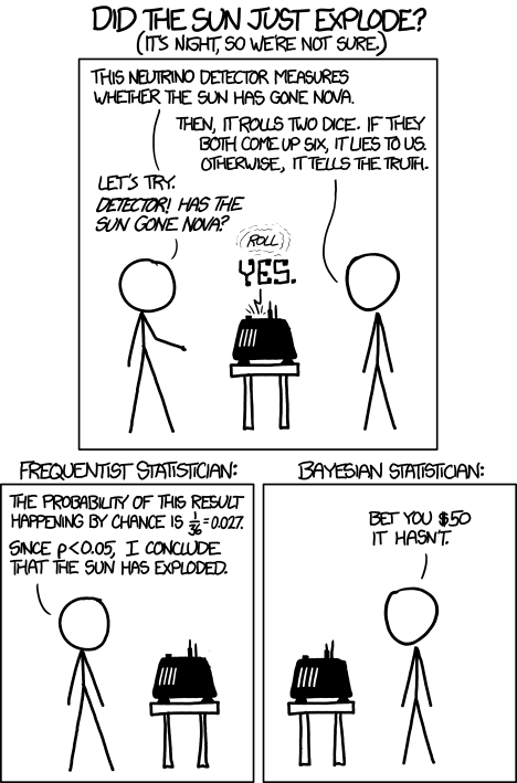
XKCD #1132: Frequentists vs. Bayesians (Randall Munroe, CC BY-NC 2.5). The Bayesian in this comic is right about priors. The Bayesian in our meeting was right about priors too. Neither of them was right about the experiment being cheap.

The proposal was reasonable and well-intentioned. My concern was specific, and asserting it without proof felt insufficient, so I brought the math.

Frequentist Sample Size

To set the baseline, here is the standard frequentist formulation. We are testing whether the rewards program (treatment) increases AV ride take-rate relative to no rewards (control), where $\theta$ is the probability a rider chooses an AV and $\Delta = \theta_T - \theta_C$ is the MDE:

$$ H_0: \Delta = 0, \quad H_1: \Delta > 0 $$

With Type I error $\alpha$ and power $1-\beta$, the required sample size per group is:

$$ n_\text{freq} = \frac{\left( z_{1-\alpha/2} + z_{1-\beta} \right)^2 \left[ \theta_C (1-\theta_C) + \theta_T (1-\theta_T) \right]}{\Delta^2} $$

where $z_q$ denotes the $q$-th quantile of the standard normal distribution. The numerator grows with the variance of each group; the denominator shrinks with the MDE squared. If the rewards program moves the AV take-rate only slightly, $\Delta$ is small, the required sample size is large, and the program runs at a loss for a long time. This was the source of the pressure: the expected MDE was small, the required sample size was large, and every additional day of the experiment was another line item.

This is the formula the Bayesian disciple proposed to improve upon. On to the proposed alternative.

Bayesian Sample Size

The Bayesian formulation replaces the frequentist error guarantees with a posterior expected loss criterion. We approximate the posterior on each group’s conversion rate as Gaussian, which is reasonable for proportions with sufficient data:

$$ \theta_C \mid D_C \sim \mathcal{N}(\hat{\theta}_C, \sigma_C^2), \quad \theta_T \mid D_T \sim \mathcal{N}(\hat{\theta}_T, \sigma_T^2) $$

with posterior variances:

$$ \sigma_C^2 \approx \frac{\hat{\theta}_C (1-\hat{\theta}_C)}{n}, \quad \sigma_T^2 \approx \frac{\hat{\theta}_T (1-\hat{\theta}_T)}{n} $$

Instead of controlling Type I error, we set a threshold $\epsilon$ on the probability of selecting the wrong group:

$$ p_\text{wrong} = \mathbb{P}(\text{choose wrong group}) < \epsilon $$

Solving for $n$, the required sample size per group is:

$$ n_\text{bayes} = \frac{\hat{\theta}_C (1-\hat{\theta}_C) + \hat{\theta}_T (1-\hat{\theta}_T)}{\Delta^2} \cdot \left[ \Phi^{-1}(1-\epsilon) \right]^2 $$

where $\hat{\Delta} = \hat{\theta}_T - \hat{\theta}_C$ is the estimated MDE and $\Phi^{-1}$ is the inverse standard normal CDF. Look at the structure. It is identical to the frequentist formula. The variance terms are the same. The MDE in the denominator is the same. The only difference is the squared prefactor: $\left[\Phi^{-1}(1-\epsilon)\right]^2$ instead of $\left(z_{1-\alpha/2} + z_{1-\beta}\right)^2$.

Example

Put some numbers on it. Suppose the baseline AV take-rate is 50% and the rewards program is expected to lift it by 2 percentage points:

• $\theta_C = 0.50$, $\theta_T = 0.52$, $\Delta = 0.02$
• Frequentist: $\alpha = 0.05$, power $= 0.8$ $\implies z_{1-0.025} + z_{0.8} \approx 1.96 + 0.84 = 2.8$
• Bayesian: $\epsilon = 0.05 \implies \Phi^{-1}(0.95) \approx 1.645$

Setting aside the variance terms, which are identical for both, the sample sizes scale as:

$$ n_\text{freq} \propto (2.8)^2 = 7.84, \quad n_\text{bayes} \propto (1.645)^2 = 2.71 $$

On paper, the Bayesian approach needs roughly a third of the frequentist sample. It is an appealing result, and the intuition behind it is sound. There is just one assumption buried in the derivation that changes everything.

Bayesian Is Not Immune to Peeking

For the uninitiated, peeking is the practice of inspecting results before the planned sample size is reached and stopping early if the numbers look good. It is what invalidates frequentist tests when p-values are checked repeatedly mid-experiment: the false positive rate inflates because you are effectively running multiple tests and keeping the best result. The same logic applies to the Bayesian posterior.

You might be tempted to think you can check the Bayesian experiment after every ride or every day. This is incorrect: you still need to let $n_\text{bayes}$ observations accumulate before evaluating the stopping criterion, otherwise this is also peeking. Bayesian methods have an additional problem here: the posterior variance can jump around quite a bit early on, so making a decision off it is unreliable. In other contexts such as the Kalman filter, this period of instability would be called burn-in.

If you evaluate $p_\text{wrong} < \epsilon$ continuously and stop the moment it dips below threshold, you have not run the experiment described by the formula above. You have run something different, with different and worse statistical properties. The Bayesian framing does not make this problem disappear. It reframes it. The stopping rule is still a rule, and it must be respected as such.

When Are the Two Formulas Exactly the Same?

The two formulas have identical structure: same variance terms, same MDE in the denominator. The only difference is the prefactor. Setting them equal gives:

$$ \Phi^{-1}(1-\epsilon) = z_{1-\alpha/2} + z_{1-\beta} $$

which means:

$$ \epsilon = 1 - \Phi\!\left(z_{1-\alpha/2} + z_{1-\beta}\right) $$

Plug in the numbers from the example above: $\alpha = 0.05$, power $= 0.8$, so $z_{1-\alpha/2} + z_{1-\beta} = 2.8$. Then:

$$ \epsilon^* = 1 - \Phi(2.8) \approx 0.0026 $$

This is what it means. For the Bayesian experiment to require the same sample size as the frequentist one, you must set $\epsilon = 0.26\%$, not the $5\%$ used in the earlier example. The apparent sample size reduction comes entirely from setting a far more lenient $\epsilon$. When you hold the error guarantees constant across both frameworks, the sample sizes are exactly equal.

It is worth noting that the relationship between $\epsilon$ and the frequentist parameters $\alpha$ and $\beta$ is not always this transparent. Under the Gaussian approximation used here, the algebra works out cleanly. For other likelihood models or more complex posteriors, deriving the equivalent $\epsilon^*$ requires its own careful analysis and the equivalence will not always take such a neat closed form. The general principle, however, tends to hold: when you account for what each framework is actually guaranteeing, no free lunch is to be found.

Conclusion

The Bayesian framework is not buying a smaller experiment. It is buying a different interpretation of the same data, at the same cost, with the same number of subsidised AV rides. If the goal is to reduce experiment duration, the honest levers are: a larger MDE (better rewards design), higher tolerance for error, or lower power. Choosing a different statistical framework is not one of them.

Appendix: Burn-In in the Kalman Filter

A Kalman filter is an algorithm for tracking a hidden quantity (say, the position of a vehicle) by combining noisy sensor readings with a prior belief about where the vehicle was a moment ago. At each time step it updates its estimate and, crucially, its uncertainty about that estimate.

The problem is that the filter needs to be initialised somewhere. If you start it with a poor guess, or simply with a very diffuse prior because you genuinely do not know, the first several estimates will be unreliable. The posterior variance is large, the estimate is sensitive to whatever noisy observation came in first, and the filter has not yet had enough data to correct itself. This settling period is called burn-in. Practitioners routinely discard these early estimates and only trust the filter’s output once the variance has stabilised.

The parallel to a Bayesian experiment is direct. In the early observations, the posterior over your treatment effect is similarly volatile, dominated by the prior and highly sensitive to the first few data points. A posterior that crosses your threshold on day two is not evidence the treatment works; it is the filter still finding its feet. Waiting for $n_\text{bayes}$ is the experiment’s equivalent of discarding the burn-in period.

References

• Robinson, D. (2015). Is Bayesian A/B Testing Immune to Peeking? Not Exactly. Variance Explained. http://varianceexplained.org/r/bayesian-ab-testing/

• Miller, E. (2010). How Not To Run an A/B Test. https://www.evanmiller.org/how-not-to-run-an-ab-test.html

• Johari, R., Pekelis, L., & Walsh, D. (2015). Always Valid Inference: Bringing Sequential Analysis to A/B Testing. arXiv:1512.04922.